home
needs
local resources
comfort
safety & health
contact
reports
Stove Control
We consider stove control from two points of view. The first one treats the woodstove as an equipment that resembles a gas stove. We call it the conventional approach. We illustrate the approach by considering the response of a typical design to changes in fuel and air supply. The approach is a theoretical one and supported by a few experimental results. The second approach explicitly makes use of the fact that wood combustion occurs in two phases - the burning of volatiles in the combustion space and the burning of char on the fuel bed. The approach is more heuristic but supported by a tailor made experiment. The approach is expected to be of use for cooking foods like beans that involve long periods of burning.
Conventional Approach: A Design Study
We have pointed out repeatedly that a major problem with wood stove designs is stove control. In this section we present a detailed investigation on a single design which will bring out the precise nature of the problem. Stove control essentially implies, in plain English, that the stove is provided with an elementary mechanical device such as a knob, a lever, or a button, which when operated will change the current power level of the fire to a new power level. If we recall that power is nothing but the burning rate of the fuel, we need to manipulate the rate at which both fuel and air are supplied to the fire for effective control.
To put things in perspective let us consider the example of a gas stove. To start the fire a knob is operated such that the maximum rate of flow of gas air mixture issues out of the burner head. The mixture is ignited by an external source of heat like a match or a spark. The burner head of a gas stove receives a premixed gas and air mixture. This does not mean that the gas pipe line supplies the gas in this form, but the stove is designed in such a manner as to adjust the air flow from the ambient according to the velocity of the gas. Higher velocities of the gas induce larger amounts of air at the inlet section of the tube at the end of which is the burner head. The distance between the inlet section and the burner head is chosen so as to permit complete mixing between air and the gas due to natural flow processes in the tube. The velocity at which the gas is supplied to the tube creates a pressure difference between the ambient and the region where the air enters. This is the pressure difference that determines the amount of air that enters the stove. The relation between the rotation of the knob and the velocity of gas entry is nonlinear. So is the relation between the velocity of gas entry and the pressure difference created which in turn is nonlinearly related to the amount of air flow. This is the reason why one notices so little variation in the flame power in the initial stages of the knob rotation.
We shall now attempt a translation of this experience to a wood re. Here we can do no better than quoting Emmons and Atreya (1983).
''The real problem arises when we wish to regulate the rate of burning to fit our needs. We of course can build a large stove or small one. The right size is not just one which can burn wood at the required maximum rate and no faster, but one which can hold a sufficient charge of wood so that it does not require recharging every few minutes.''
''But here is the major difficulty. Suppose a charge of wood able to supply the required heat overnight can be accommodated in the stove. What is to prevent the fire from growing very rapidly throughout the wood supply and consuming it in the first few hours? We cannot control the internal energy transfers between sticks and thus control the fire growth. The only practical control is the air supply. Thus dampers (valves in the air supply system) are used to adjust the air flow. ''
''This controls the rate of fire growth all right. However, it does so by preventing the rapid burning of charcoal and by controlling the heat release in the flames. This reduces the energy feedback to the fuel, thus reducing its pyrolysis, which is what we wanted. However, the control of the heat release in the flames was accomplished by supplying insufficient air to burn all the fuel.''
There appears to be an inconsistency in the above line of argument. If the pyrolysis rate is reduced, it is reasonable to expect that less volatiles come to the flame region and as such the air supplied must be sufficient to burn the volatiles efficiently. However the response of the pyrolysis rate to the change in the heat release rate in the flames is poorly understood. Under these conditions the designer has to merely fall back on well tested and tried ideas and hope that the research community will come up with a satisfactory answer to this question one of these days.
There is an important difference between the heating stove that Emmons and Atreya were considering and the cook stove that the present work is about. The average household cook stove is rarely operated for more than a couple of hours at a time. Secondly the cooking task is such that the cook is required to be present in the stove vicinity for most of the time. Thus the demands placed on the system are not that stringent in the case of cook stoves as they are in the case of heating stoves. These factors imply that one need not consider charge sizes that need last much more than twenty minutes or so. In spite of these differences the limitations of the type indicated by Emmons and Atreya are still operative as we shall demonstrate in this section on the design study.
We will carry out the study on a single pan chimney stove. We will choose the chimney Mai Sauki (see above). The speci fcations of the design are provided below according to the drawing shown in Fig.2 (Bussmann 1988).
The pan
Dp = 27.7 cm
h1 = 19.5 cm
h2 = 9.0 cm
The pan can hold 8.1 litres of water when it is filled to the brim.
Pdes = 4.8 kW
Expected efficiency = 35%
The stove dimensions
D8 = 297 mm
Hdes = 220 mm
Combustion chamber
dc = 170 mm
hc = 100 mm
Fuel loading opening
shape: triangle
Hf = 110 mm
W f = 115 mm
area = 57 cm2
Chimney
diameter = 70mm
height = 300mm
entrance = 70*50mm2
Air Holes
shape: rectangular
size: 25*50 mm2
number: 4
total area: 50 cm2
The stove was not provided with any special control mechanisms.
As can be seen from the above list the stove is indeed a very simple device for fabrication. A kerosene wick stove - which is ostensibly produced by the informal sector industry - is a much more complex apparatus and thus this sector should be able to produce this wood stove without too much difficulty. There are three methods of control available for the designer.
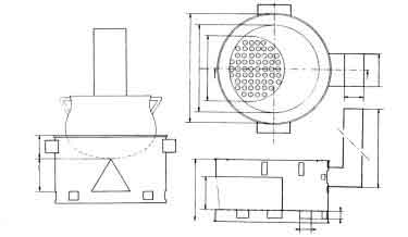
Fig.1. The Chimney Maisauki
(i) The first method concerns the situation as intended by the designer. It provides for only one type of control - the alteration of fuel charge size. The question here is: will the system adjust itself in such a manner that the burning rate will reduce and a corresponding reduction in air flow will occur?
(ii) The second is to alter the air flow into the system by introducing an appropriate resistance, that can be varied at will a la the knob in the gas stove, in the flow path. The question here is: will the burning rate adjust itself to the new air flow rate?
(iii) The third method will simply use a combination of the methods (i) and (ii) above.
We shall investigate only the methods (i) and (iii) in some detail with reference to the chosen design since there are no simple methods available to estimate the consequences of changing just the air flow without altering the charge.
In order to proceed with a quantitative description we shall make a few assumptions. Firstly the wood used is taken to be oven dry white fir with a heating value of 18.7 MJ/kg. For the design power of 4.8kW the burning rate turns out to be
Taking the ultimate analysis of the fuel to be C: 0.50; H: 0.06; and O: 0.44 by weight, we can calculate the air flow rate, with an excess air factor of 2, for the design power to be
Thus the combustion gases generated in the system will be simply the sum of wood burnt and the air supplied and will be
We shallnow estimate the pressure drops and the draught generated in the system by the formulas introduced earlier.
The Inlet Resistance
This was calculated by Bussmann (1988); but he ignored the possibility of air flowing through the fuel loading door. We shall explicitly take thisinto account. Noting the three features recommended by the designer, namely:
(i) the fuel door is triangular;
(ii) the wood sticks are of size 30mm in diameter; and
(iii) there can be accommodated three sticks in the first layer and two sticks z in the second layer
and making the further assumption that the user will never let the fuel in the bottom layer burn out, we can estimate an average area available for air ow through the fuel loading opening (see Figure 10.20) as
This could be thought of as the secondary air to the fire. The primary air is supplied through the air ports mentioned earlier in the design speci cations and comprise of four rectangular ports of an area
each. In order to calculate the total resistance offered by this system of air flow it is handy to use the electrical analogy indicated in the Figure 3.
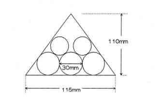
Fig.2 . The fuel loading opening area available for air flow
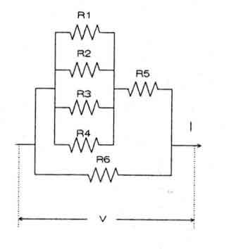
Fig.3. Electrical analogy of resistances offered by the inlet area
In the above diagram the resistors R1 to R4 could be combined according to
Since in our design all the inlet ports are of equal area and discharging into the same enclosure the resistors R1 to R2 are equal to one another and denoting it by R, we have
Now Req and R5 are in series and R6 is parallel to them. We can write the total inlet resistance by following the same procedure as above
In the above R6 denotes the resistance to secondary air flow and R5 the resistance offered by the grate -fuelbed combination. The data presented earlier should be considered as preliminary for use in design work. The other source of information is ow through packed beds commonly used in many chemical industries. These are invariably for very high mass ow rates and it is doubtful whether they can be used for such low ow rates as we encounter in our case. In the absence of de nitive data we simply assume
Rt then becomes
Once Rt is known the voltage drop across the system can be calculated as
In analogy with this we can write
Comparing the two expressions we note
Following this analogy we can write expressions for R, R6, and
Rtleading to the following expression for the inlet pressure drop
![]() .
.
In the above expression we know all the quantities and
![]() is taken to be 0.6. Thus the pressure drop across the inlet ports including the fuel
loading opening is (note that the density of air has to evaluated at the
ambient temperature from a table of properties, say from Eckert & Drake,
1972; in the calculations presented below the ambient temperature has been
taken as 300 ° K.
is taken to be 0.6. Thus the pressure drop across the inlet ports including the fuel
loading opening is (note that the density of air has to evaluated at the
ambient temperature from a table of properties, say from Eckert & Drake,
1972; in the calculations presented below the ambient temperature has been
taken as 300 ° K.
Sudden enlargement
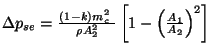
The next cause for the pressure loss is the sudden enlargement that occurs in our stove between the combustion chamber and the stove body (see gure 1). The pressure loss across a sudden enlargement is given by the expression (10.17). We can rewrite the expression in terms of areas and the mass ow by noting that
This leads to the following expression for the pressure loss across the sudden expansion.
 (17)
(17)
Every quantity in the above expression is known except
![]() which depends on temperature. The simplest method to estimate the temperature is
to use the following expression.
which depends on temperature. The simplest method to estimate the temperature is
to use the following expression.
The trouble with this expression is that cp the specific heat at
constant pressure is also a function of temperature. If a computer is being
used for the calculation it is easier to fit a curve for the values of cp
from a table of properties. If hand calculations are being done the
tables have to be directly used. Whichever is the equipment used the best
approach to calculate Tc is to use an iterative procedure. Qc
is simply the power output of the fire, which is for the present stove 4.8kJ/s
minus the losses through the combustion chamber walls which in the present
case happens to be double walled. The heat balances given for
the so called experimental stove show that this loss cannot be more than
15% if we note in the present design the combustion chamber height has been
deliberately chosen low. This implies that Qc is 0.85 of 4.8kJ/s. This
leads to a value of Tc and a corresponding
![]() from the table of properties. k can be read from Table 10.7. All this effort leads to
from the table of properties. k can be read from Table 10.7. All this effort leads to
This is really less than 1% of the pressure loss at inlet and for all practical purposes can be ignored. That is the characteristic of the design we have chosen. In particular when lot of air goes through the system as many a current stove design permits, then this can be important. Of course the interest in the present development is to establish the critical points at which the pressure drop occurs. Thus in the rest of the work we shall ignore this pressure drop.
The chimney pressure loss
There are three separate elements to the chimney calculation. In this particular design an obstruction is provided at the entrance to the chimney, again deliberately to hold the air flow through the stove to the desired level. The second element consists of a bend. The final element is the chimney itself. Before we do the loss calculation we must know the temperature at the entrance to the chimney. It can be calculated by Eq.(10.23) using exactly the same procedure except Qch needs to be estimated with care.
From an energy balance we can see that
The first term on the right hand side has been estimated. Qs is the stove
body loss from the end of the combustion chamber to the top of the stove
bodywhich we simply set equal to the combustion chamber wall loss, that is,
15%. Qi is the heat input and is 4.8kJ/s.
![]() is the efficiency and has been estimated to be 35% by the designer. Thus we obtain
is the efficiency and has been estimated to be 35% by the designer. Thus we obtain
Following the same procedure as we did with Eq.(10.22), we obtain
Cp;ch = 1:091kJ/kgK (22)
We are now in a position to calculate the various pressure losses. The first one is the obstruction. Treating the obstruction as a gate valve, we can use Table 10.8 and Eq.(10.18) for the geometry indicated at the beginning of this section to obtain the k factor as 0.44.. The velocity through the chimney can be obtained from Eq.(10.21). Thus the chimney entrance pressure loss is
The second item is the bend. We can use Table 10.8 for this purpose. We need to choose r=d -this really depends upon the space availability. For the design we are considering it can be taken to be 1. is taken to be 90 degrees which is true for most chimney installations. From the table k is seen to be 0.22. The pressure loss in the bend is thus
The last loss in the chimney is the friction loss in the straight section. To estimate this we make use of Eqs.(10.12), (10.13) and (10.14). The Reynolds Number turns out to be 1680. This is in the laminar ow regime and calculate the friction loss factor from Eq.(10.13) which works out 0.0381. Using these in Eq.(10.12), we get
The total pressure loss in the system is simply the sum of all the individual pressure losses and is
Finally we can calculate the chimney draught from Eq.(10.10).
The draught is somewhat smaller compared with the pressure drop and thus the excess air factor will be smaller than designed. This may have adverse consequences on the stove performance. The natural question is: by how much will the air supply decrease? For an estimation of this we can use Eq.(10.20), which can be rephrased as
 (30)
(30)
For our design this results in a little under 7% decrease in airflow which can be considered as acceptable since we have an excess air factor of 2. In this formulation a major assumption has been made. The density is treated as a constant which is not true. This effect has to be carefully accounted for larger differences and one has to recalculate and obtain the actual effect.
The description provided so far has concentrated on the design point. We now turn to the control aspect or what is commonly known as off design performance. The first method was to simply reduce the rate of availability of fuel. Before embarking upon the detailed calculations we will provide a heuristic picture of what can happen. For the sake of illustration let us say that we wish to reduce the power by half. The way this is done is that one usually starts the stove at full power operation and when the flames have stabilized (probably some 10 to 15 minutes after the fire has been started) the reduction in the power is undertaken by reducing the fuel charge by half. Since in principle the same amount of air is going through the system, one would expect a lower Tc with the consequence that Tch is also reduced. It follows therefore that the draught will get reduced. The efficiency tends to fall with increased excess air, with an attendant increase in Tch. Thus the reduction in draught will not be as much as anticipated by the previous effect. We will now provide some numerical estimates for this type of control.
We make several assumptions while deriving the estimates of off-design performance of the stove. We list them below.
(i) We can vary the charge size at will. Note this is the only means we have at our disposal for changing the power from the fire in the current design.
(ii) The above increases the free area available through the fuel loading opening for theair ow. This is estimated on the basis of the wood size recommended by the designer.
(iii) The losses from the combustion chamber and the stove body are taken to be directly proportional to the power of the fire. In other words the loss coefficients are invariant with the power of the fire.
(iv) The efficiency values, required to estimate the heat carried away by the chimney gases, do not change very much. There at least two reasons for this behaviour. Firstly as the power is lowered the re becomes more compact and essentially the ame heights tend to become smaller. This tends to reduce the efficiency. On the other hand the excess air factor increases with reduction in the power of the fire which in turn tends to increase the ame height. This acts counter to the first effect .
The actual values are those obtained by experiments on the shielded fire .
Armed with these assumptions we can calculate the stove behaviour when we change the power of the fire. The strategy we adopt in the calculation is to let the total air flow in the system remain unchanged as the power of the fire is varied. At the end we compare the total pressure drop in the system with the available chimney draught. This can be used to verify our strategy of assuming that the air flow through the system is invariant.
This table shows some remarkable properties of the wood fires. We began with the assumption that the air ow does not change by changing the power output. A superficial look at the problem suggests that the reduction in the heat release rate ought to be accompanied by a corresponding reduction in the intake of air. In fact if we look at the rows 16 and 17, barring the design situation, in all the other cases the chimney draft is much higher than the pressure drop across the stove. In other words, as we reduce the power of the fire more air gets sucked into the stove than was the case with full power. This extra air reaches a value of about 13% for the lowest power shown (see row 18) in the table.
The reason for this behaviour is easy to deduce if we trace our path back a little. At first we note that in principle have two pressure drops - one at the inlet and the second at the chimney. The only factor that changes at the inlet is the area of the fuel loading opening due to smaller charges employed. It is easy to show from Eq.(10.20) that
| 1. | P, kW | 4.8 | 3.6 | 2.4 | 1.6 |
| 2. | mfx104,kg/s | 2.57 | 1.93 | 1.28 | 0.87 |
| 3. | ma x104 ,kg/s | 30.65 | 30.65 | 30.65 | 30.65 |
| 4. | mc x104 ,kg/s | 33.22 | 32.58 | 31.94 | 31.51 |
| 5. | charge, g/900s | 240 | 160 | 120 | 80 |
| 6. | As x104,m2 | 18.7 | 24.35 | 30.0 | 36.2 |
| 7. | 1.70 | 1.24 | 0.93 | 0.69 | |
| 8. | Tc, ° K | 1320 | 1110 | 875 | 700 |
| 9. | Efficiency, % | 35 | 33 | 30 | 28 |
| 10. | Tch, ° K | 765 | 680 | 575 | 500 |
| 11. | Vch, m/s | 1.896 | 1.652 | 1.370 | 1.18 |
| 12. | Re | 1680 | 1700 | 1960 | 2120 |
| 13. | 0.36 | 0.31 | 0.25 | 0.21 | |
| 14. | 0.18 | 0.15 | 0.13 | 0.11 | |
| 15. | 0.13 | 0.11 | 0.079 | 0.06 | |
| 16. | 2.37 | 1.81 | 1.38 | 1.07 | |
| 17 | 2.08 | 1.91 | 1.63 | 1.37 | |
| 18. | mc,c /mc,d | 0.94 | 1.03 | 1.09 | 1.13 |
| 19. | 2 | 2.67 | 4 | 6 |
Thus as the area increases the pressure drop falls as the square of the area. At the chimney we can express the pressure drop by
From Eq.(10.22), we see that
Thus
In the above we have ignored the small change in the mass flow of the
combustion as a result of reduced burning rates. Since
![]() is inversely
proportional to the temperature, we conclude from the above that the
pressure drop at the chimney strictly follows the temperature at its
entrance. As we see from row 10 of the table the temperature at the entrance
to the chimney continuously falls and so do the pressure drops as can be
seen from the rows 13, 14, and 15 when we reduce the power. Finally we see
the principal conclusion of the analysis -the excess air goes on increasing
from 2 to 6 as we reduce the power by a factor of 3.
is inversely
proportional to the temperature, we conclude from the above that the
pressure drop at the chimney strictly follows the temperature at its
entrance. As we see from row 10 of the table the temperature at the entrance
to the chimney continuously falls and so do the pressure drops as can be
seen from the rows 13, 14, and 15 when we reduce the power. Finally we see
the principal conclusion of the analysis -the excess air goes on increasing
from 2 to 6 as we reduce the power by a factor of 3.
We have made very many heroic assumptions while developing the arguments above. It seems reasonable to determine whether these arguments have any basis on what is actually observed in stoves in actual operation. Unfortunately there are very few pressure measurements in stoves. But a few gas analysis measurements are available on a very similar stove, the Tamilnadu Stove that can be used to determine the excess air. There is one major dfference between the two designs though. The Tamilnadu stove has a door closing the fuel loading port. In spite of it, it is worthwhile taking a look at these results since the role of the chimney in both cases should be similar. Table 2 shows the results of a few experiments for which gas analysis was available.
The results clearly show that the chimney temperature falls and the excess air factor increases as the power output of the re decreases. Note the rather high efficiencies of this stove and they change very little with the power output. Correspondingly the chimney temperatures are low.
A second piece of evidence comes from a two pan mud stove -the Tungku Lowon from Indonesia. It is chimneyless with an open fuel loading port. The result is shown in Table 2.
| Sl. No. |
P kW |
Efficiency % |
Tch °K |
Flue Gas Composition (%) |
|||
| CO2 | CO | O2 | |||||
| 1. | 10 | 50 | 472 | 10.3 | 0.7 | 10.9 | 2.079 |
| 2. | 7 | 51.4 | 437 | 9.1 | 0.36 | 13.8 | 2.917 |
| 3. | 3.6 | 54 | 413 | 6.5 | 0.35 | 14.5 | 3.231 |
Source:Sulilatu et al. 1985
| Sl. No. |
P kW |
Efficiency % |
Tch °K |
Flue Gas Composition (%) |
|||
| CO2 | CO | O2 | |||||
| 1. | 6.88 | 17.9 | 486 | 12 | 1.81 | 7.34 | 1.60 |
| 2. | 4.20 | 20.6 | 469 | 10.62 | 0.83 | 9.85 | 1.9 |
| 3. | 3.30 | 21.6 | 478 | 8.16 | 0.78 | 12.01 | 2.42 |
| 4. | 2.1 | 20.8 | 430 | 4.3 | 0.28 | 16.7 | 4.62 |
Source: Claus et al (1983)
Again it is seen that the excess air increases significantly with the reduction of power output. These two examples provide adequate evidence to support the type of calculation we have presented in Table 10.12.
The major difficulty lies with the size and species of the wood used. The designer recommends a 3cm diameter wood and a maximum of 5 pieces of wood per charge. We note that the diameter of the combustion chamber is 17cm. We take this as the e ective burning length of wood in the stove irrespective of the length of the sticks used. Thus at full power the amount of wood participating in combustion per charge is 600cm3. Since the experimental results we have quoted are all for white fir, we use its density of 400kg=m 3 to obtain the weight per charge to be 240g. This will burn in about 15 minutes at the full power. At thelowest power it has to use only 80g per charge or one and two-thirds of one stick in the above period. This does not seem unachievable.
We will now see the effect of changing wood species. Consider for example using species such as Eucalyptus camaldulensis or Tamarindus indica with a density of over 900kg/m3. Such woods will weigh per charge of ve sticks 540g. The burning rate demands that the charge period will increase to about 34 minutes. We will immediately get into the Emmons-Atreya syndrome we started this section with. Moreover at the lowest power we need to burn just 3/4 of a stick in the charge period. Thus an open fuel loading port system can never manage to do these things e ectively.
We will turn now to the question of controlling the air flow to the stove. The intention is to control the air ow through the stove such that the excess air factor remains uniform whatever be the power level of the re is. This suggests a strategy to adopt to calculate the flow behaviour of the stove. We simply let the excess air remain constant and carry out the computation which will provide us the necessary guideline to evaluate the additional resistance (adjustable of course) to be introduced. Before getting on with the presentation of the results one or two brief remarks over the positioning of the resistance need to be made. In principle in the current design two places are available -one at the air inlet and the second at the chimney. The air control at the inlet will not work (see later). In the present design we shall use a chimney damper. The results of the computation are presented in Table 3.
Rows 1 to 17 need no explanations as they have been covered while discussing Table 10.11. Row 18 is the extra pressure drop to be supplied by the control mechanism. In the table we have chosen a butter y valve in the chimney. If the valve to chimney diameter ratio is taken as 0.8, we will not be able to obtain control down to the one-third of the power. It will supply the correct air amounts up to little over half power. The rest of the power range has to be organized through the mechanism of simply using smaller charges. On the other hand, if we choose the above ratio to be 0.9 we get the requisite control and more. But there is a catch here. The gap between the chimney and the damper would be 3.5mm. This requires a much superior production technology than is feasible for most production systems that are currently in use in West Africa.
A natural question that follows this presentation is: why not introduce the control mechanism at the inlet? It can be easily demonstrated by using Eq.(10.21) that this is a non-starter for the quantities of air flow and pressure drops required. It simply demands the closing of the fuel loading port.
The second type of question arises with respect to the height of the chimney. In the design we have been investigating an ultra short chimney has been used. There are three reasons for this choice. The design was developed for use in a Sahelian country, especially Niger, where considerable proportion of the cooking takes place outdoors. Thus the purpose of the chimney is not one of providing for better indoor air quality but preventing the smoke directly hitting the face of the cook while she is manipulating the food she is cooking. Secondly an important criterion for the acceptance of the design was that the stove be portable. This constrains the height of the chimney to about 50cm.
Finally there is the all important question of cost. Whatever is said and done there is no getting away from the fact that a chimney is very expensive. Under certain conditions its cost can equal or exceed that of the stove body (see later).
Nevertheless it is worthwhile taking a look at taller chimneys since these are invariably used with multi-pan mud stoves which are xed devices in the kitchen. While we will not repeat the calculation for a multi pan stove (same methodology can be used; see here for the estimation of flow resistances in the ASTRA stove).we shall simply demonstrate what can happen with the Mai Sauki. We shall satisfy ourselves by just quoting some results for full power condition (see Table 4).
| 1. | P, kW | 4.8 | 3.6 | 2.4 | 1.6 |
| 2. | mf x104, kg/s | 2.57 | 1.93 | 1.28 | 0.87 |
| 3. | ma x104, kg/s | 30.65 | 22.99 | 15.33 | 10.26 |
| 4. | mc x104, kg/s | 33.22 | 24.91 | 16.61 | 11.07 |
| 5. | charge, g/900s | 240 | 160 | 120 | 80 |
| 6. | As x104, m2 | 18.7 | 24.35 | 30.0 | 36.2 |
| 7. | 1.70 | 0.70 | 0.23 | 0.09 | |
| 8. | Tc, ° K | 1320 | 1328 | 1328 | 1328 |
| 9. | Efficiency, % | 35 | 35 | 35 | 35 |
| 10. | Tch, ° K | 765 | 765 | 765 | 765 |
| 11. | Vch, m/s | 1.896 | 1.42 | 0.95 | 0.63 |
| 12. | Re | 1680 | 1260 | 840 | 560 |
| 13. | 0.36 | 0.20 | 0.09 | 0.04 | |
| 14. | 0.18 | 0.10 | 0.045 | 0.02 | |
| 15. | 0.13 | 0.10 | 0.067 | 0.04 | |
| 16. | 2.37 | 1.02 | 0.43 | 0.19 | |
| 17 | 2.08 | 2.08 | 2.08 | 2.08 | |
| 18. | 1.059 | 1.64 | 1.88 | ||
| 19. | Chimney damper | ||||
| kr | 2.3 | 8.04 | 20.7 | ||
| dda = d ch = 0.8 Position, ° |
37 | 68 | 20.7 | ||
| ddda = d ch = 0.9 Position, ° |
29 | 47 | 63 |
Notes:
(i)
(iii) dda: damper diameter; (iv) Positions of the damper obtained by interpolation from Table 10.8.
| 1. | Chimney Height, m | 0.3 | 2.0 1st app |
2.0 2nd app |
| 2. | 1.70 | 1.70 | 7.87 | |
| 3. | 0.36 | 0.36 | 1.05 | |
| 4. | 0.18 | 0.18 | 0.58 | |
| 5. | 0.13 | 0.75 | 1.71 | |
| 6. | 2.37 | 2.99 | 11.19 | |
| 7. | 2.08 | 13.89 | 9.76 | |
| 8. | mc,c / mc,d | 0.94 | 2.16 | 0.93 |
| 9 | 2.0 | 4.31 | 4.03 |
It is useful to start with a couple of comments on the calculation presented above. The first approximation simply assumes that the increase in chimney height only in uences the chimney friction loss and the draught. There is a great deal of imbalance between the total pressure drop and the draft. We have used the new quantity of air that is inferred by and recalculated all pressure drops. It is instructive to see that while our books balance better, it does very little to the total air ow through the system -a mere seven percent change from the starting value. It is obvious to see from the above table that enormous amounts of air go through the system as the chimney height isincreased.
We examine a few choices one has to fix things properly.
(i) The first choice is to reduce the chimney diameter. Two consequences of this are a change in the chimney velocity and a corresponding change in all the losses. For example reducing the chimney diameter to 0.05m from 0.07m increases the total losses to 9.798 Pa. This results in a 19% increase in air ow over the starting value we used.
(ii) A second option is to constrict the ow much more at the entrance to chimney. For example, in Table 10.8 reducing the value of h=D to 0.3 increases the total resistance to 10.812 Pa. The increase in air ow will be about 13% -clearly does better than the first option.
(iii) The final option is to reduce the size of the inlet port. If we have no inlet ports and air can come in only through the fuel loading port the total resistance will be just 4.49 Pa. This results in a 75% increase in flow -clearly is no option.
It is obvious that a combination of the first two options with proper dimensioning of the chimney diameter and the constriction at the chimney entrance will lead to an excess air factor around 2 whatever be the height of the chimney be.
We have presented considerable amount of calculations in the foregoing. We repeat the earlier reservation that they are based on many assumptions. The coefficients we have used come from mostly air conditioning practice. There is also no mention in these tabulations of the ow Reynolds Number e ect. We expect this to be small. However we are calculating small pressure drops. How does one safeguard against these uncertainties? There is only one method -the time honoured one of experimentation. The time is ripe at this stage of design to construct a prototype of the design. The testing programme should cover several power levels of the re. At a minimum the water boiling eÆ ciency, the gas temperatures at the bottom and the exit of the chimney (note in our work above we have used only the entrance chimney temperature for our draft and density calculations; it is preferable to use the average temperature and thus the suggestion), and gas analysis need to be measured. These will provide adequate information to test the various assumptions made in the work presented here.
An Alternative Approach
We have already made an inventory of the cooking tasks that one encounters in practice. In the list presented there, boiling dry food in water is the most important. Therefore in the following discussion we will restrict ourselves to the cooking of food with water as the medium. At the end of the section some references will be made to the other food-cooking processes.
Generally, boiling in water proceeds in two phases: first there is a high power phase in which the food and water mixture is brought to the boil; the only demand of the process on the stove is a high power, so the time to bring the food to the boil is short. The second phase is the simmering phase. The requirements of the process made on the stove in this phase are much more strict: the stove must be able to operate at a low enough power to keep the content of the pan boiling without evaporating too much water. Evaporation is a thermal loss and it increases the danger of burning the food. From the descriptions in Section on cooking tasks and the Section on Fuel Economy, it is clear that a stove is required to deliver a high power, followed by a low power. This is the principal function of control in a stove. To make the control effective the time constant connected with the controlling action must be small compared to the process time; so for cooking this has to be of the order of a couple of minutes. We will illustrate the nature of the control problem of a stove by considering the cooking of lentils. They require a simmering time of 1 hour when they have received no prior preparation. For a 5-kg water equivalent of the mixture and an efficiency of 30%, a 4-kW fire will bring the mixture to a boil in 23 min. The power level requirement for the simmer phase is very small: one needs to keep the mixture just at the boiling point. Thus only the heat losses from the pan have to be compensated. For a covered and reasonably well-shielded pan, these losses will be no more than 1000 W/M2 (98), leading to a loss of 115 W for a pan to cook this amount of food in. Assuming that the efficiency at power levels this low is about 20%, the power requirement is just 575 W.
The wood requirement for this can be easily calculated. Assuming air- dried wood with a calorific value of 15 MJ/kg, 368 g is needed for the boiling phase and 138 g for the simmering phase. But these calculations implicitly assume a constant power from the wood fire. However, since wood is not available on tap, the fire must be charged at reasonable time intervals with reasonable-sized wood blocks. Say 160 g of wood is charged every 10 min to get the 4-kW fire. Then the volatiles will be burnt in approximately 9 min, and the charcoal in 10 min. The resulting power curve is shown in Fig. 59.
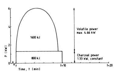
Fig.X.
To achieve the low power we encounter problems. With reasonable sized fire wood, a fire of 575 W is impossible. The minimum possible power will be between 2 and 2.5 kW and ways to achieve these low powers are also limited: the charge weight or the charge intervals can be reduced.
Changing the charge weight offers the possibility of charging, for instance, 50 g at intervals of 6 min. This is considered undesirable: a fire like this asks too much of a cook's attention. Using the same charge weight of 160 g, then the charge intervals must be 16 min for a nominal power of 2.5 kW. Because the volatile power is the same (see Open fires), the power curve now will look like Fig. 60.

Fig.X-1.
It. can be seen from this curve why no lower power is possible, and further that there is a high power phase, which will keep the food mixture vigorously boiling for 9 min, and a low power phase in which the temperature will drop below the boiling point. For each of the successive charges this will be repeated. The evolution of volatiles, which can not be controlled in an open fire, is the cause of this. One could think then of a closed stove with air control, but it is argued by Verhaart [16] control of the volatiles evolution is unlikely to work through the control of air flow. Probably there exists a feedback cycle: less air-> less flames -> less radiation to the fuel -> less volatiles. This mechanism has not yet been investigated and surely is worth further research. But as far as we can presently see, the time constant of such a scheme would be too large to be useful for cooking purposes. But a closed stove with air control offers another interesting possibility: the control of the burning of charcoal that remains after the volatiles have burnt. Then the behaviour of the wood fuel and the demands of the boiling of food can be matched to the following possible solution: for the part of the cooking scheme that requires high power, the volatites are burnt; for the part that requires low power, the remaining charcoal is burnt. To do this we need a stove with separated primary and secondary air flows, both controllable. This is realised in a modified version of the shielded fire, already mentioned in Section V. The stove can be operated as follows. In the high power phase, the primary air damper is closed and the secondary air damper is fully opened. In this way the volatiles in the wood are burnt and the charcoal remains on the grate for later use. The fire is charged at high power charging intervals, with charges as big as possible.
At the moment the desired temperature is reached, the secondary air damper is closed and the primary air damper opened to start the burning of the charcoal at the desired power, just enough to keep the food simmering. This procedure is illustrated by the application of the calculation procedure developed earlier in this section.
The premises are as follows. A 5-kg water equivalent is to be brought to a boil. We use wood as fuel, and the heat of combustion is 18730 kJ/kg. The stove efficiency is 40% for a power range of 6-3 kW. This wood is assumed to have a charcoal content of 20% and a volatile content of 80%. The fire is charged with 143 g of wood every 8 min, giving a nominal power of 5.6 kW.
First only volatiles are burnt. The volatile power is 3.6 kW. For an efficiency of 40%, 1.44 kW goes into the pan. For this situation the water starts boiling after 19.5 min. Over these 19.5 min three charges of 143 g are fed into the stove, so the high power volatile phase lasts for 24 min. These three charges produce a charcoal bed of 86 g of charcoal.
From experiments we know that for low powers the stove efficiency is about
25%, and a power of about 400 W is needed to keep the water boiling. The 86
g of charcoal represents 2838 kJ. Burning at 400 W, this amount of fuel will
last for 118 min. We can compare these results with the data obtained from
experiments on this type of shielded fire (see Table 6).
| Pnom (kW) |
Tb (min) |
Tsim (min) |
Wc (g) |
Psim (kW) |
|
| Calculation | 5.6 | 19.5 | 118 | 86 | 0.400 |
| Experimental | 5.6 | 22 | 68 | 78 | 0.774 |
Tb = time to boil
Tsim = simmering time
Wc = initial weight of charcoal bed at start of simmering phase
Psim = simmering power
For the high power phase the calculations match very well with the experimental results. The results for the simmering phase differ because the power was twice as high as the one in the experiment. But the calculated amount of charcoal on the grate at the beginning of the simmering phase matches the calculated amount, 86 versus 78 g. In this case the primary air damper was closed to 50% in the beginning and closed to 25% at 70 min. We see that shortly after that moment the power reduces to 0.350 kW, and also the water temperature drops below 100 ° C.
Figure 61 gives the relevant graphs on the same time scale. This gives occasions to some more remarks. The second charge did not burn too well. This is one of the interesting and frustrating things about a woodfire: although we try to normalise fuel, experimental procedures, and circumstances, the behaviour is never uniform. General predictions can only be done for the average of a number of experiments. The number of experiments that have been done on this stove is very small, so the only thing that can be said now is that it holds promise.
The next thing Fig. 61 shows is that a charcoal bed burns constantly, governed by the amount of combustion air, as long as it has a thickness exceeding a certain minimum value. After that the amount of charcoal itself becomes the governing variable for the power.

Fig.X.
Although experimental support is still poor, the idea of using the fuel- wood volatiles for a high power phase and the charcoal for a low power phase offers possibilities for reduction of fuel consumption and fire control over the low power phase. The period over which the food can be kept simmering with the charcoal saved over the period of bringing the food to a boil will be sufficient for most foods. Fuel consumption rates in ternis of kilograms of wood per kilograms of food of 0.4315 = 0.086 are possible and a careful operator can reach even lower values.
Finally, we want to make some remarks about other cooking processes. Some of them also have a high power phase to start with, but followed by a moderate power phase to finish the cooking, for instance deep-frying. Others need a moderate power from the beginning, for instance deep frying. This type of stove offers possibilities for all these cooking processes. A number of experiments have been done on a shielded fire without air control, using the same kind of fuel blocks (32 x 32 x 1 10 mm). Smaller blocks are difficult to contemplate at the user's level. These experiments have shown that a power range of 6 kW down to 2 kW is possible only by controlled fuel supply. With air control we are able to burn charcoal in a power range of 0.3-1 kW. Lower powers are not needed because then boiling will stop. Thus there is a gap in the power range between 1 and 2 kW. More experiments need to be done to see if this gap in the power range can be covered. As the stove is now, the distance between pan bottom and grate is tuned to flaming combustion. Setting it at an intermediate height between the optimal for flaming and charcoal combustion could mean an improvement over the whole scale of cooking schemes. But the possible effects on combustion quality should be looked into with great concern, as the discussion in Section on Indoor Air Quality will point out.