home
needs
local resources
comfort
safety & health
contact
reports
Performance Estimation of Stoves
Subsections
Introduction
In other pages of this website we have tried to develop a level of understanding of stoves - be they the traditional open fire or what are known as improved stoves - based on a mixture of theoretical models and laboratory experimentation. These form the basis on which new designs of stoves suited to diverse situations that arise in practice could be worked out. Since this understanding cannot be considered foolproof , one ought to have a satisfactory procedure for assessing the performance of a design. While we have discussed the various experimental techniques elsewhere, these were done primarily with a view to understand the processes in a cookstove and thus useful for research situations in a reasonably well-equipped laboratory. But cookstoves have to be used in kitchens operated not necessarily by research engineers with plenty of time and facilities. Thus designs need to take these into consideration explicitly.
The difference between the laboratory situation and a practical situation has often been posed in such a manner as to suggest that the laboratory work cannot provide any guidelines for the development of efficient stoves. It is claimed that only field work can lead to practical designs. Our aim is here to reconcile these two world views and show both types of work are essential for developing successful designs.
Over the years many testing procedures have been suggested, all of them claiming to be the best way to establish the performance of a stove, and trying to express that performance by a single number usually referred to as ``the efficiency''. But the system of a woodburning cookstove is too complex to be captured by one number. The components of the system are the operator, the fuel, the pan-stove combination, and the food to be cooked. Each component has its input to the system and influences the result. So performing tests on the whole system is very complex and will produce results that are very difficult to interpret. A better approach then is to test parts of the system and try to combine them to produce results applicable for the whole system. The first component that is sacrificed is the operator. She/he is replaced by a precisely described procedure of feeding the fuel into the stove. The second sacrifice is the food to be cooked. This is replaced by water. The real food-cooking tests are limited to a validation of the results obtained by water-boiling tests. This leaves us with the system of fuel and pan-stove combination. How can we express the performance of this system in comprehensible terms?
A natural question in this connection is what do we mean by performance of a stove? We use the word to denote collectively:
- (i)
- the power output of the fire;
- (ii)
- the range of power output;
- (iii)
- the efficiency;
- (iv)
- the ease of starting;
- (v)
- tar formation and/or stove emissions;
- (vi)
- maintenance; and
- (vii)
- life expectancy.
In this list the efficiency is the most discussed item among cookstove workers, and its definition has caused great deal of confusion. One of the remarks often heard is ``we are not per se interested in the efficiency, but in the fuel consumption of a stove.'' It is easy to see that fuel consumption is the product of the efficiency, power output, and the time over which stove is used. It appears to the author that there is an inadequate appreciation of the problem among the purveyors of such statements.
To put things in perspective let us consider a simple example. Consider the problem of cooking rice. The mixture of rice and water has to be brought to boil (most cooks would like to have this phase completed in a rather short time); the mixture must simmer thereafter with the lid closed. The former step will require the greatest feasible power output from the stove and the latter will require the lowest possible power output - just enough to make up the heat losses from the pan - to maintain the mixture at or near boiling temperature. In fact, the second phase could be carried out in a hay box - a well-insulated enclosure to attain nearly zero heat loss from the pan. Thus the fuel consumption for the operation is determined by
- (i)
- the efficiency, whose usual definition is the ratio of heat absorbed by the food to the heat supplied by the fire at the two power output levels used in the operation; and
- (ii)
- the actual power output levels.
A stove that is not capable of delivering low enough power output levels for simmering operations (which can be particularly long for cooking lentils and different types of dried beans) will inevitably show large fuel consumption.
But the call for fuel consumption figures persists partly because the procedure to convert efficiency information to fuel-consumption information is not well developed. That is one of the principal tasks of this section. Before that we shall present a detailed critique of the so-called water boiling tests in order to establish its validity for determining the efficiency of a cookstove. We shall then present measurements and analysis to establish the minimum power required to keep the contents of the pan at or near boiling temperature. This is treated under the heading control.
We then present methods to establish heat balances in stoves. The purpose of the section is to provide insights into the areas one needs to concentrate on for improving the efficiency of a system. There is another important concern, namely, the response of a stove to fuel change. This is important since the users do not get the same type of wood always and hence it is useful to have some idea about the extent of changes in the performance one could expect under these conditions. This is considered in the section on fuel type (See the Block Diagram on Design)
A Critique Of Efficiency Measurements
As mentioned earlier there exist a number of different test procedures. In the early eighties representatives of the two groups representing field and laboratory practitioners agreed on a provisional international standard for the testing of the efficiency of woodburning cookstoves (VITA, 1982). The standard describes a water boiling test (with two alternatives), a controlled cooking test, and a kitchen performance test. It also gives a method for conversion of water-boiling test results into wood consumption values. The standard carries the marks of a marriage between two opposed interests, and has unecessary drawbacks for laboratory work. Since that time there have been many national standards (for example in India, China, Sahel, to name a few). It is not the intention here to reproduce these standards. Most of them are based on water boiling tests with slight variations. In this section we shall provide a detailed analysis to assess the reliability of a water boiling test to provide efficiency values. We will restrict ourselves here to the practice followed in the water boiling test used to obtain many of the efficiency results and compare it with the VITA standard referred to earlier.
Bhatt (1983) throws more light on the efficiency measurement by different procedures. He defines eight testing methods. Without going into many details, we shall indicate the broad idea behind his test procedures.
- (i)
- Water boiling tests as used in the earlier sections .
These will be discussed in greater detail later on in this section. - (ii)
- Constant heat output method
Khanna (1975) and Micuta (1985) recommend this procedure. It consists in bringing a definite quantity of water to a high temperature, such as 96 ° C, and repeating it with successive batches of water in similar vessel (vessel type is not explicitly specified at least by Bhatt), presumably till all the wood in the stove is used up (again this is left vague by Bhatt). The heat absorbed by water is simple to calculate if the initial temperature and mass of water is known. The amount of wood used can be measured and if one knows the moisture content and the calorific value of the wood used, the heat input for accomplishing the job can be calculated leading to an efficiency value. - (iii)
- Constant temperature rise method
This is said to be a modified version of the Indian Standard for electric stoves and is considered suitable for constant power output stoves. A fixed quantity of water is heated through a temperature rise of, say 20 or 30 ° C and the time to accomplish this is noted. The test is repeated several times and an average time to accomplish the task is computed. Since time and power is known one can compute the energy input. The heat absorbed by water is easy to evaluate. Thus one gets the efficiency. - (iv)
- Constant time method
This is a modified version of the method (iii) above. It attempts to heat a fixed quantity of water over a fixed interval of time and note the temperature rise. The experiment is repeated several times and an average temperature rise is computed. The efficiency value follows from a calculation of the type mentioned in (iii). - (v)
- Cooking simulation tests
These will be discussed in extenso later on. - (vi)
- Process simulation tests for large stoves used in small
scale industries
There are a variety of products made in such stoves. We name two: jaggery (unrefined sugar) processing stoves; and dolo (a sort of beer) production stove in Sahel. Again the test generally follows the lines of cooking simulation tests. - (vii)
- Indirect method
In large scale cooking establishments, it is not feasible to estimate the efficiencies easily. Bhatt proposes an indirect test. The energy input is estimated by performing the task on either a scaled version or full scale on an electric stove. The efficiency is estimated. From the users of such stoves wood consumption is obtained. Comparison of the energy consumption in the electric stove test with the latter gives an estimate of the efficiency of the large stove. - (viii)
- Approximate method
This is what one could call a ``quick and dirty method'' proposed by Bhatt. This is applicable to large installations where the stove is in continuous use. If the user can spare something of the order of 15 minutes a known quantity of water is heated during the period and the temperature rise of the water is noted.
Bhatt used as many of these methods as possible to test several classes of wood-fired appliances:
- (i)
- cook-stoves and boilers;
- (ii)
- special-purpose stoves for areca-nut boiling, jaggery making, and making beaten rice;
- (iii)
- stoves for parboiling paddy, liquor distillation, and fabric dying.
We shall not go into the detailed results for all the different types of stoves, but present the results obtained by him for cook stoves and water boilers (see Table 1). Method (v) - the cooking simulation test - is the one that gives consistently lower values. It appears from the description provided by Bhatt that the conditions of the tests were not the same as those in the other testing procedures. Looking at the other procedures it appears that there can be upto 50% difference among the procedures in a relative sense. If we omit the cooking simulation result the simple water boiling test provides generally a conservative estimate of the efficiency of the stove. Bhatt concludes the following from his work.
- (i)
- To determine cookstove efficiency strictly from its design considerations, irrespective of the user's capacity for utilizing the output heat energy, the water-evaporation method may be used.
- (ii)
- To determine the combined performance of a cookstove, based on its design considerations as well as the user's capacity for utilizing the heat output, the cooking-simulation test may be used.
- (iii)
- To assess the user's capacity for uitlizing the output heat energy irrespective of stove performance, the efficiency ratio may be used, i.e., the ratio of the efficiency as determined by the cooking-simulation test to that by the water-evaporation method (both measured at the same power output level). This test must be conducted while the users are operating the stove.
The water-evaporation method used by Bhatt is the same as that used for results reported in this work. About this method, Bhatt concludes; ``For cookstoves, the water-evaporation method is convenient and accurate.''
Although water-boiling tests are a convenient and accurate way to test a
stove, the measurement technique must be well defined in order to produce
reliable and accurate results, because the process and the variables
concerned are not as simple as they may look at first glance.
| Stove type | Testing | P o | |
| Method | (kW) | (%) | |
| Three stone stove | (i) | 3.5 | 10.7 |
| (process temperature | (ii) | 3.3 | 8.9 |
| = 100 - 190 ° C) | (iii) | 3.8 | 13.7 |
| (iv) | 3.6 | 12.9 | |
| (v) | 3.7 | 5.7 | |
| (vii) | 3.5 | 9.5 | |
| (viii) | 3.4 | 12.2 | |
| Portable mud stove | (i) | 3.0 | 16.8 |
| (process temperature | (ii) | 3.2 | 14.2 |
| = 100 - 190 ° C) | (iii) | 3.6 | 18.2 |
| (iv) | 3.3 | 18.6 | |
| (v) | 3.0 | 6.3 | |
| (vii) | 3.1 | 14.0 | |
| (viii) | 3.1 | 15.7 | |
| Two-pot opening stove | (i) | 4.5 | 12.3 |
| (process temperature | (ii) | 3.9 | 9.2 |
| (iii) | 4.4 | 16.7 | |
| (iv) | 4.9 | 15.8 | |
| (v) | 4.6 | 6.2 | |
| (vii) | 4.2 | 12.7 | |
| (viii) | 4.9 | 14.1 | |
| Bath water heater | (vi) | 21.8 | 15.9 |
Efficiency in thermal systems is a concept derived from the application of the first law of thermodynamics. It is simply the quotient of output and input of a device performing a well-defined task. For a woodburning stove the input is the wood energy used up in the stove and the output is the cooked food. Both these quantities are not easy to measure in a wood-burning cooking stove as the following discussion will reveal.
First let us consider the measurement of input energy. There are two important features of woodburning systems that make this difficult. The first feature is concerned with the fact that a solid fuel device of the capacity we are considering is a batch process system. In other words, the fuel is not available on tap, but an operator has to load the fuel into the stove and keep on doing this at frequent intervals. The number of refueling operations can be large. This makes it difficult to monitor the system's input with a sufficient degree of reliability. In most traditional practices, wood is invariably used in long peices. In cooking situations, the wood keeps on burning and one is required to push the wood pieces at frequent intervals of time so that the fire is always kept under the pan. Thus the procedure is equivalent to the batch process.
The above feature has another important implication. The efficiency, as pointed out earlier, is derived from the first law of thermodynamics. This law does not explicitly involve time as an independent variable. For continuous systems, the law is used by defining a steady-state operation. Such a mode of operation is not easily realized in a batch system. The best one could hope for is to consider the stove to be in steady periodic operation. Ideally such a situation could be realized in a stove by adding small charges of wood at fequent intervals (say every 5 min). After the first three or four charges, steady periodic operation will be established in the system. While this is not difficult to achieve in the disciplined environment of a laboratory, it is hardly to be recommended for use in a kitchen. Thus it is to be expected that practical systems will be working in a time-dependent manner. The best that can be done is to measure either an average heat input or an overall heat input over a defined period of time. The latter is the quantity measured in most of the presently available literature on the subject.
The second feature concerns the fuel quality. The latter is used here as a catchall phrase to denote wood species, the as-fired moisture content in the wood, and the size of the wood actually employed in the stove. All these factors are highly variable in practical situations and may strongly influence the heat output of a given stove design.
Added to these rather natural complications of the fuel used, there is yet another difficulty - a completely man-made one. Many a stove designer claims that his design can burn any fuel. What he means by this is that his design will accept all kinds of fuels so long as they are solid. Specifically what he means is that you can load these into his stove, and burn them after a fashion. Saying this is one thing and it is quite another to say that all these fuels provide the same amount of heat output from a given design. If the design is any good at all, it will provide the best performance for one fuel. Other fuels, when used, will yield performances that depart from optimal performance depending upon the departure of the fuel characteristics from the design fuel. This departure could be minimized by processing other fuels. For instance, sawdust, firewood chips, and agricultural waste can be pressed to form briquettes. We shall look at this question in detail towards the end of this page. We will reject the stoves that are designed without taking the fuel characteristics into consideration as unreliable.
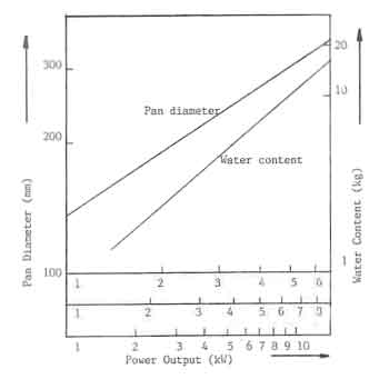
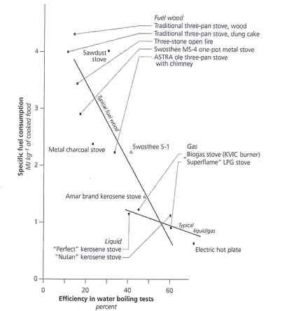
We now turn to the measurement of the output. The quantity of the energy transferred to the water in the pan(s) on the stove has to be measured. This task is less complicated than the measurement of the input, in the sense that we have to deal with quantities that are easily measurable: temperatures and weights. Because the physical properties of water we need - the specific heat and the heat of evaporation - are well known, we can calculate the output with an accuracy that is far better than the accuracy with which the input can be established. But there is a choice to be made about what pan is to be used for the test and how much water this pan must contain, since significant efficiency variations can be obtained by varying the pan size. The problem was recognized a long time ago by the testers of gas stoves, and the V.E.G. Gas Institute in The Netherlands uses a rule of thumb for gas ranges. Their recommended heat flux through the pan bottom is 3.5 W/cm 2. At an efficiency of 50% this requires a power density at the pan bottom of 7W/cm 2. For wood stoves since the efficiencies are much lower, the power densities can be much larger. Thus Fig.1 which shows this relation, has been drawn for three different scales along the x-axis corresponding to power densities of 7, 10 and 17.5W/cm 2 for efficiencies of 50, 35 and 20% respectively. The reason for the choice of 3.5W/cm 2 is that the normal aluminium pans used in Europe are unable to withstand higher heat fluxes.
With this graph we can select a suitable pan for a given stove. Still the results will be valid only for this specific pan-stove combination. The next question concerns the quantity of water to be used for the tests. The V.E.G. Gas Institute also recommends the heights to which the pans are to be filled for testing. This is also shown in Fig.1. But it is not possible to determine any rationale for this recommendation. The earlier mentioned Provisional International Standard for testing woodstoves (VITA 1982) states that two-thirds of the pan should be filled with water for water-boiling tests. This is a reasonable recommendation as long as no data are available on the influence of the degree of filling on the efficiency.
Altogether, water-boiling tests appear to be not that simple, or, stated otherwise, we are trying to test a complicated system. Only a sharply defined test procedure can produce reliable results, and the more straight-forward this procedure is, the better. This is where the problem arises with the international standard mentioned earlier. Basically this standard recommends the following procedure for a water-boiling test:
- (i)
- Take quantity of wood not more thant twice the estimated needed amount.
- (ii)
- Start the fire at high power to bring the water in the first pot (the major concern in developing a procedure here was multi-pan stove; thus this reference to the first pot) to a boil and keep it boiling for 15 minutes.
- (iii)
- Note the time; remove all wood from the stove, knock off any charcoal, and together with the unused wood from the previously weighed supply weigh all the charcoal separately, record the water temperature from each pot, weigh each pot, including water and lid, and return charcoal, burning wood, and pots to the stove to begin the ``low-power'' phase of the test.
- (iv)
- Continue the test at a low power, so that the temperature of the water stays within 2 ° C of boiling. Continue for 60 minutes using the least amount of wood possible.
- (v)
- Recover, weigh, and record separately the charcoal and the wood; weigh and record the remaining water in each pot.
These results are used to calculate the Standard Consumption as a figure to express the quality of the stove and to compare different stoves. The reason to perform a test like this is that it provides a fuel-consumption figure, which is more appealing to the people who will have to buy these stoves in the future. The efficiency concept as the ratio between input and output is too abstract and has been misused in the past. While this is true, but it is important to recognise that this way of testing is too complicated for the following reasons.
- (i)
- Recovery of the charcoal is not sharply defined and is therefore operator dependent. The charcoal weights are small and measurement of such small weights is always subject to large errors.
- (ii)
- Estimation of the combustion value of charcoal, produced in a wood fire is at best a tricky task.
- (iii)
- A lot of things must be done in as short a time as possible between the high-power and the low-power phase, so the risk of making mistakes or misreadings is pretty high.
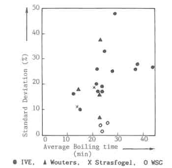
Concluding, it is reasonable to state that this way of testing cannot be expected to produce very reliable results unless one uses sophisticated instrumentation and great care in the conduct of the experiment and measurement. Bussmann (1988) assembled test results from different sources using the above procedure on 19 different stoves covering nearly 180 tests and compares them with the water boiling tests used in obtaining the results at Eindhoven. The measured boiling times were used as the test parameter for comparison. The results are shown in Fig.2.
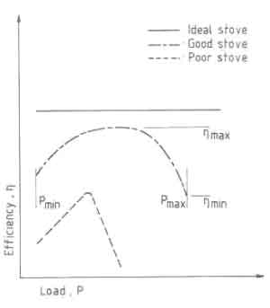
The test described above is basically a cooking-simulation test with the water replacing the food, and tries to fulfill the needs of both field workers and lab workers. The authors believe that for laboratory work on wood-stove research and development a more engineering-oriented attitude must be taken. Thus it is useful to compare the woodstove with some standard engineering equipment, say for example the centrifugal water pump (Krishna Prasad 1981). A woodstove can be characterized by an efficiency-versus-power geaph. Figure 3 gives an example of how such a graph might look for an ideal, a good, and a poor stove. The efficiency figures for a pan-stove combination should be established by steady-state water-boiling experiments (corresponding to method (i) of Bhatt mentioned above). For woodstoves, the best we can hope for is periodic steady state. And the waterboiling test then is no longer a simulation of food-cooking process, with the water replacing the food, but instead the measurement of a heat transfer process, with the water as a convenient medium to measure the heat transfer from the fire to the pan. The procedure adopted for the results quoted in this work has been found through experience to be very simple and extremely reliable. It consists of a few simple instructions:
- (i)
- Plan the experiments to last upward of an hour or burn 1 Kg or more of wood; to vary the power output under the batch opertion system simply divide the total fuel quantity to be used in the experiment into five or six equal parts and charge the stove at intervals of time determined by the desired power output; thus the air-dried. wood considered above produces approximately 5 kW if 200 g of wood is charged into the stove every 10 min.
- (ii)
- See that all the wood burns; the indication for this is the drop in water temperature below boiling point.
- (iii)
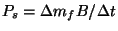
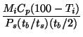
- Weigh the water before and after the experiment. Efficiency can then be calculated by Eq.1
where the symbols are: ![]() , efficiency; Mi, initial mass of water (kg); Cp specific heat of the water (J/kg K);
Tb, boiling temperature of the water (K);
Ti, initial temperature of the water (K);
me,evaporated amount of water (kg);
, efficiency; Mi, initial mass of water (kg); Cp specific heat of the water (J/kg K);
Tb, boiling temperature of the water (K);
Ti, initial temperature of the water (K);
me,evaporated amount of water (kg);
![]() , specific heat of evaporation (J/kg);
mf, mass of fuel burnt (kg); and
Bw, combustion value of the wood (J/kg).
, specific heat of evaporation (J/kg);
mf, mass of fuel burnt (kg); and
Bw, combustion value of the wood (J/kg).
- (iv)
- Curves of the type shown in Fig.3 can then be generated in a few days work.
The objections against the procedure would be that it does not adequately represent the cooking procedure. The author's contention is that it does not matter. Once a graph of the type shown in Fig.3 is obtained, it is possible to estimate the fuel consumption for a specified cooking operation (see next section). This estimate can then be verified through actual cooking tests. So here the formation of steam is taken as useful output of the system. It is a positive result of the heat transfer, while in the efficiency definition of a cooking process, steam formation must be considered as a loss.
The final question that remains is the relationship that exists between the steady-state efficiency defined above and the efficiencies obtained with water-boiling tests, which were not conducted with a view to determine the steady-state performance. As such, an exact value for this efficiency cannot be obtained. An attempt is made below to estimate this efficiency on the basis of some assumptions. This will be followed by certain comments on these assumptions to establish reliability of these estimates.
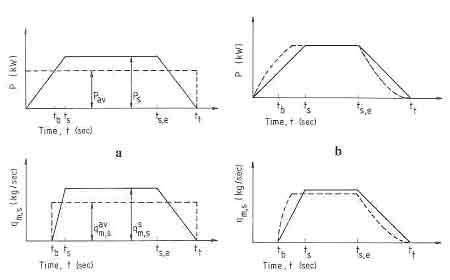
The analysis is based on the model shown in Fig.4 dividing the burning of a woodfire into a buildup phase, a steady periodic phase, and a decay phase. In Fig.4a, tt is the total burning time and tse is the product ofnumber of charges and period between two successive charges. This is taken as the end of the steady periodic regime; t s is the beginning of the steady periodic regime and t b
- (i)
-
 , i.e., the buildup of the fuelbed takes the
same time as its decay;
, i.e., the buildup of the fuelbed takes the
same time as its decay; - (ii)
- the buildup and decay of the fuelbed occur linearly; and
- (iii)
-
 (2)
(2)
where is the mass of charge (kg),
 is specific combustion value of fuel (J/kg),
 is charge interval (s), and
 is steady-state mean power of the fire (W).
Similarly with regard to steam generation, the following additional assumptions have been made:
- (i)
- there is no evaporation before boiling point is reached;
- (ii)
- when
 ,
a linear buildup of rate of steam generation to the steady-state level of
,
a linear buildup of rate of steam generation to the steady-state level of
 (kg/sec);
- (iii)
- when
 , an instantaneous buildup of rate of steam
generation to
; and
, an instantaneous buildup of rate of steam
generation to
; and - (iv)
- a linear decay of
to
 .
.
This model can be used to evaluate the steady-state efficiencies for the system as follows. We first note that
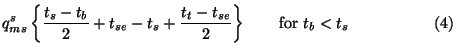 |
|||
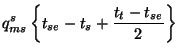 for for
|
The steady-state efficiency is then defined by
 (6)
(6)
where ![]() is the latent heat of evaporation of water (kJ/kg). The results so obtained for a number of
experiments (Krishna Prasad 1981) are presented in Tables 2 and 3. In these tables values of
is the latent heat of evaporation of water (kJ/kg). The results so obtained for a number of
experiments (Krishna Prasad 1981) are presented in Tables 2 and 3. In these tables values of
![]() are the efficiencies calculated by Eq.(6). All the efficiencies correspond to first-pan results.
Two important observations can be made from a comparison of
are the efficiencies calculated by Eq.(6). All the efficiencies correspond to first-pan results.
Two important observations can be made from a comparison of
![]() and
and
![]() .
First,
.
First, ![]() <
<
![]() for every case tabulated except for run number 151 in Table 2 and run number 60 in Table 3. The
actual departure of
for every case tabulated except for run number 151 in Table 2 and run number 60 in Table 3. The
actual departure of
![]() from
from
![]() in
Table 2 ranges from 1.6 to 13.7% based on
in
Table 2 ranges from 1.6 to 13.7% based on
![]() with an average of 8.2%. Similar results have been obtained for the family cooker. According
to the model proposed, there is not an enormous departure of
with an average of 8.2%. Similar results have been obtained for the family cooker. According
to the model proposed, there is not an enormous departure of
![]() from
from
![]() and the method followed in our work produces acceptable results.
and the method followed in our work produces acceptable results.
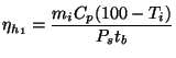
In order to ascertain the validity of the assumptions made in the model,
efficiencies for the warming-up period were calculated as follows:
 for for
|
(7) | ||
 for for
|
This is compared with
![]() calculated by
calculated by
 (9)
(9)
| P | |||||
| Run no. | (kW) | (%) | (%) | (%) | (%) |
| Charge: 4 pieces | |||||
| 71 | 4.37 | 18.9 | 18.3 | 19.6 | 22.3 |
| 70 | 6.56 | 16.9 | 16.1 | 13.3 | 21.3 |
| 75 | 7.76 | 19.0 | 18.3 | 18.2 | 22.6 |
| 74 | 8.74 | 17.5 | 15.9 | 17.0 | 25.8 |
| 151 | 9.61 | 18.3 | 19.3 | 12.2 | 15.4 |
| 69 | 10.8 | 16.3 | 14.9 | 13.1 | 33.1 |
| 73 | 13.3 | 14.5 | 13.1 | 11.7 | 36.7 |
| Charge: 6 pieces | |||||
| 109 | 5.35 | 17.0 | 15.7 | 20.9 | 25.8 |
| 110 | 6.45 | 17.3 | 17.0 | 15.7 | 18.5 |
| 123 | 7.46 | 16.2 | 14.9 | 15.9 | 21.1 |
| 111 | 8.30 | 16.4 | 15.0 | 14.9 | 25.0 |
| 153 | 9.41 | 17.9 | 15.9 | 16.7 | 37.6 |
| 108 | 10.3 | 14.8 | 13.3 | 14.4 | 25.4 |
| Charge: 8 pieces | |||||
| 138 | 5.58 | 16.4 | 15.3 | 18.1 | 21.6 |
| 156 | 6.60 | 17.4 | 16.2 | 17.6 | 23.8 |
| 107 | 7.28 | 15.6 | 14.1 | 17.8 | 27.6 |
| 137 | 8.06 | 15.5 | 14.5 | 13.9 | 21.1 |
| 106 | 11.2 | 15.1 | 13.4 | 15.1 | 20.7 |
| 136 | 12.2 | 14.5 | 12.8 | 12.8 | 45.7 |
In Eqs. (7)-(8), mi is the initial mass of water,
Cp is thespecific heat of water, and
Ti is the initial temperature of water. The
results are again displayed in Tables 2 and 3;
![]() is reasonably close to
is reasonably close to
![]() while
while ![]() shows considerable departures. In particular, for cases where
shows considerable departures. In particular, for cases where
![]() ,
the departures are by as much as a factor of 2 or more. These findings provide a clue as to
the nature of the approximations involved.
,
the departures are by as much as a factor of 2 or more. These findings provide a clue as to
the nature of the approximations involved.
There is little reason to doubt the validity of Eq.(1) and as such the
existence of a steady periodic regime. Thus the errors in estimates of
![]() (which is our principal interest) can only arise by the method of estimating
(which is our principal interest) can only arise by the method of estimating
![]() .
The error in
.
The error in ![]() can arise due to three factors.
First, we have ignored the evaporation rates during the warming-up period.
For all practical purposes this source of error can be ignored. Second, and
probably most serious, is the assumption that
can arise due to three factors.
First, we have ignored the evaporation rates during the warming-up period.
For all practical purposes this source of error can be ignored. Second, and
probably most serious, is the assumption that
![]() .
.
| P | |||||
| Run no. | (kW) | (%) | (%) | (%) | (%) |
| 47 | 4.7 | 24.3 | 23.4 | 22.6 | 45.1 |
| 64 | 4.7 | 19.0 | 18.4 | 18.3 | 36.6 |
| 44 | 4.7 | 18.8 | 18.4 | 18.9 | 37.8 |
| 60 | 4.7 | 14.7 | 16.2 | 13.3 | 26.6 |
| 45 | 4.7 | 15.9 | 15.4 | 17.3 | 34.5 |
| 50 | 6.3 | 19.8 | 17.8 | 18.2 | 36.5 |
| 48 | 6.3 | 17.6 | 14.6 | 16.8 | 33.6 |
| 49 | 6.3 | 16.0 | 14.4 | 14.6 | 29.2 |
| 62 | 6.3 | 16.4 | 14.7 | 15.1 | 30.2 |
| 51 | 6.3 | 13.6 | 12.1 | 12.2 | 24.3 |
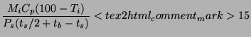
where
The constants represent the combustion value and conversion factor to convert kilowatts to kilojoules.
The effect of changing this assumption is illustrated in Fig.3b. It has only
a marginal effect on
![]() but a substantial effect on the fuel consumption estimates for the warming-up period.
Third, the linear assumption of decay and buildup of fire is also suspect.
In this connection it is to be remembered that
but a substantial effect on the fuel consumption estimates for the warming-up period.
Third, the linear assumption of decay and buildup of fire is also suspect.
In this connection it is to be remembered that
![]() and
and
![]() are to be held constant. This leads to the conclusion that the heat liberated
during the buildup and decay of fire should be equal. In other words, these
processes can be quite different and these can easily account for the unduly
large efficiencies during the warm-up period.
are to be held constant. This leads to the conclusion that the heat liberated
during the buildup and decay of fire should be equal. In other words, these
processes can be quite different and these can easily account for the unduly
large efficiencies during the warm-up period.
The main conclusions to be drawn from the above exercise are that:
- (i)
- the model proposed here produces reasonably correct estimates of steady-state efficiencies for the system;
- (ii)
- the general method for determining efficiences used in our work produces results that are in close agreement with the true steady-state efficiencies;
- (iii)
- there is no reason to believe that large quantities of steam produced in experiments of this type produce artificially high efficiencies; in fact, the efficiencies during the warm-up period will be higher than those for the boiling period; and
- (iv)
- the large efficiencies obtained for the warm-up period, particularly at high powers, are suspect; provided the experiments are carried out for a sufficiently long time, these have only marginal influence on steady-state efficiencies.
These somewhat conjectural arguments require experimental support. The experiments need to measure at the minimum the water weight loss at virtually the same intervals as the charging intervals.
Efficiency and Fuel Economy
In the preceding discussion we have argued that it is not necessary to perform cooking tests on a woodstove in order to establish wood consumption figures. Simple water-boiling tests are very convenient and accurate way to make up a graph of efficiency versus power for a given pan-stove system. And we have shown that the testing procedure suggested above produces efficiency figures that are close to the periodic steady-state figures one ideally would like to use for such a graph. Still, what we have to do is to convert the efficiency figures to wood consumption figures. In the following analysis a calculation procedure will be presented that does this job with reasonable accuracy, which will be shown by comparison with existing food-cooking data. Further, the method will be used to make clear how important it is to develop stoves with a wider power range or turn-down ratio than there exist now. First we will present the calculation method as developed by Krishna Prasad et.al. (1983).
Theory
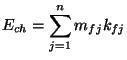
The energy required to cook n food ingredients in a medium
![]() can be conveniently split up into five component parts.
can be conveniently split up into five component parts.
- (i)
- Energy required to raise the medium from the ambient to the
cooking temperature
where m m is the mass of the cooking medium (kg), Cpm is thespecific heat of the cooking medium (J/kg K), Tm is the cooking temperature (K), and Ti is the initial temperature (K).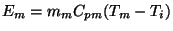 (10)
(10)
- (ii)
- Energy required to raise the food ingredients from ambient
to cooking temperature
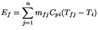 (11)
(11)
where mfj is the mass of food ingredient j (kg), Cpj is the specific heat of food ingredient j (J/Kg K), j is the subscript for different food ingredients, and Tfj is the cooking temperature of the food (K). We would like to draw attention to Tfj it can be differentfrom Tm (see Verhaart (1983) for a discussion in connection with the preparation of French-fried potatoes). - (iii)
- Energy used up for the production of water vapor
 (12)
(12)
where me is the mass of evaporated water (kg), is the latent heat of evaporation of the cooking medium (J/kg), and
me has to be
determined by weighing the food and medium before and after cooking. The
water vapor could be formed either from the medium (when it is water or milk
or some other dairy product) or from food ingredients (in particular,
vegetables, meat, and fish have large quantities of water in them). Thus
most of the cooking processes will involve the production of water vapor
whatever the cooking medium may be.
is the latent heat of evaporation of the cooking medium (J/kg), and
me has to be
determined by weighing the food and medium before and after cooking. The
water vapor could be formed either from the medium (when it is water or milk
or some other dairy product) or from food ingredients (in particular,
vegetables, meat, and fish have large quantities of water in them). Thus
most of the cooking processes will involve the production of water vapor
whatever the cooking medium may be. - (iv)
- Energy absorbed by the chemical process that accompanies
cooking
 (13)
(13)
where kfjis the specific chemical energy necessary for the conversion of raw into cooked food. - (v)
- Energy to make up for the heat losses from the pan We
cannot give a formula for this quantity, but we will give an estimation
later on in connection with the discussion on minimum power output of a
stove.
El - energy to make up for the heat losses from the pan
Thus the total energy required for the completion of a cooking task is given by
This expression shows that mf is reduced by increasing
![]() but also by reducing
but also by reducing
![]() .
Both these can be to a great extent influenced by the stove design.
.
Both these can be to a great extent influenced by the stove design.
We only use one value for
![]() here, because for a properly designed and operated woodstove the efficiencies at the high-
and low-power ends are close to one another. In cases where these two efficiencies deviate
too much from each other, the formula to be used would be
here, because for a properly designed and operated woodstove the efficiencies at the high-
and low-power ends are close to one another. In cases where these two efficiencies deviate
too much from each other, the formula to be used would be
where ![]() is high-power efficiency and
is high-power efficiency and
![]() is low-power efficiency. In Eq. (16), Ech and Ef
are independent of the stove design, but are determined by the quantity
and chemical/physical properties of the food to be cooked. However,
Em and El are strongly influenced by the stove design
as the discussion below will demonstrate.
is low-power efficiency. In Eq. (16), Ech and Ef
are independent of the stove design, but are determined by the quantity
and chemical/physical properties of the food to be cooked. However,
Em and El are strongly influenced by the stove design
as the discussion below will demonstrate.
To be able to perform these calculations, we will have to collect data for the different energy-consuming terms. We will restrict the discussion to situations where water is the cooking medium. In fact, water is the principal cooking medium for a large number of dishes in the world. Because the physical properties of water are known, calculating Em and Ee is not a problem. As to the total mass of cooking medium needed, we must make one more remark. The total mass of cooking medium m m consists of the amount we expect to evaporate, me , and the amount to be absorbed by the food to be cooked. This latter can be expressed as a multiple of the mass of food to be cooked. According to Verhaart (1983), these multiplication factors are 1.5 for rice and 1.44 for lentils. To calcuate Ef we need the specific heat of the food ingredients. These are reproduced from Geller and Dutt (1983) in Table 4.
| Moisture content | Specific heat | |
| Food | (% wet basis) | (kJ/kg K) |
| Rice | 10.5 - 13.5 | 1.76 - 1.84 |
| Flour | 12.0 - 13.5 | 1.80 - 1.88 |
| Bread | 44.0 - 45.0 | 2.72 - 2.85 |
| Lentils | 12 | 1.84 |
| Meat | 39.0 - 90.0 | 2.01 - 3.89 |
| Vegetable oil | 1.46 - 1.88 | |
| Milk | 87.5 | 3.85 |
| Carrots | 86.0 - 90.0 | 3.81 - 3.93 |
| Onions | 80.0 - 90.0 | 3.60 - 3.89 |
| Potatoes | 75 | 3.51 |
| Apples | 75.0 - 85.0 | 3.72 - 4.02 |
For Ech, the chemical energy needed to convert raw food into cooked
food, numerical data are hard to come by. What we do know, however, is that
this energy is small compared to the other energy terms. For instance, for
rice the chemical conversion energy is 176 kJ/kg according to Geller and
Dutt. Getting ahead of our calculation, the results show that for cooking
1kg rice on an average stove (Pmax = 4 kW, Pmin = 2 kW,
![]() = 35%) the total energy input from the fuel must be 5980 kJ. Of this
amount the 176 kJ for the chemical conversion represents only 3%, which is
negligible. Generally stated, the chemical energy is used to bind the
absorbed water. The chemical energy is more or less proportional to the
amount of absorbed water during cooking, so the above estimation for rice
will also hold for other foods. In our calculations we neglect
Ech.
= 35%) the total energy input from the fuel must be 5980 kJ. Of this
amount the 176 kJ for the chemical conversion represents only 3%, which is
negligible. Generally stated, the chemical energy is used to bind the
absorbed water. The chemical energy is more or less proportional to the
amount of absorbed water during cooking, so the above estimation for rice
will also hold for other foods. In our calculations we neglect
Ech.
The last term is E1
, which covers the heat loss from the pan.
This heat loss is dependent on many factors and we will provide an estimate
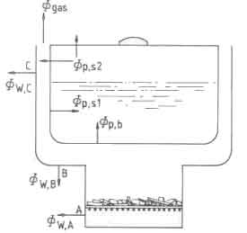
for this in what follows. Figure 5 shows heat flows into and from the pan
located on the top of a stove. the bottom of the pan receives heat while the
lid (or top surface of the food mixture when there is no lid) loses heat.
The pan side is more difficult question (see Experimental Techniques). The
pan side for the stove designs considered here is covered by the rising hot
gas column from the combustion zone. This gas cools down as it rises due to
two reasons: heat transfer to the pan and entrainment of cold air from the
surroundings. it is quite possible that at some point Yp along
the pan (see Fig.5) the temperature will fall below that of the pan. Thus
the pan side below Yp will receive heat, but above Yp
will lose heat. The exact location of Yp is too cumbersome to
estimate and we will be satisfied with some ballpark estimates. DeLepeleire
and Christiaens [1983] estimated that the heat loss from an aluminum lid will
be 700 W/m2. Noting from Fig.8 that the temperature difference
driving the heat transfer will be lower for the pan side, and further that
not all the area of the pan side may be losing heat, the pan side heat loss
may not be higher than 350 W/m2. On these assumptions Table 4 has
been constructed for the heat losses from different pans.

| Sl. | Pan size (cm) | Heat loss | |
| No. | Diameter | Height | (W) |
| 1. | 14 | 7.5 | 22 |
| 2. | 16 | 8.5 | 29 |
| 3. | 18 | 10.1 | 38 |
| 4. | 20 | 11.0 | 46 |
| 5. | 24 | 12.6 | 65 |
That these figures are reasonable can be concluded from the results of DeLepeleire and Christiaens, for cooking tests on pans standing on an insulating surface. For a pan 26 cm in diameter and with a height of 23 cm (with lid), a heat loss of 168 W over a temperature drop from 100 to 95 ° C was estimated. If the lid loses 700 W/m2 then the sides must lose 697 W/m2. Because this is for pan sides that are not enveloped by hot gases, as is a pan on a stove, our estimate of 350 W/m2 is reasonable. Really, for our calculation it is not so important if this estimate is reasonable because this heat loss is incorporated in the efficiency figure established with the water-boiling test.
With this information we can perform the calculation, of which an example will be worked out below. But first we want to express another criticism on the provisional international standards for testing the efficiency of woodburning cookstoves [VITA 1982]. The procedure presents a method to calculate wood consumption figures from the water-boiling test results. The basic idea behind the calculation is the same as is used here, except the heat for the chemical reactions is ignored, which is reasonable as pointed out earlier. But the amount of water that is absorbed by the food during cooking is ignored. Further, the standard takes the specific heat of the food equal to the specific heat of water. The influence of these errors is opposite directions, so they partially make up for one another, but in principle the method is wrong. And again the standard mixes up two thoughts: first it describes water-boiling tests that are simulations of a cooking process, and then it uses these results to calculate fuel consumption for an arbitrarily defined cooking process!
A simplified version of the formula (15) was derived by Bussmann et al.(1985) with the following assumptions.
- (i)
- The cooking medium and food ingredients are replaced by the
concept of water equivalent defined by
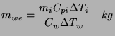 (16)
(16)
- (ii)
- The efficiency for the heating and simmering phase is the same; and
- (iii)
- The temperature rise is taken to be 75 ° C.
Then there results for the specific fuel consumption (SFC) the following expression.
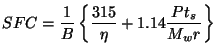 kg of fuel/kg of water equivalent of food cooked (17)
In this exprebssion Mw, the mass of water equivalent includes the loss
of water due to evaporation,
![]() is the ratio of Pmax and Pmin (the so-called
turn-down ratio) and ts is the simmer time in seconds.
The expression shows some remarkable features of the specific fuel
consumption. There are two parts to the expression. The first part
representing the heating part is independent of the power output of the
fire. This is a natural consequence of the first law of thermodynamics which
does not take note of the time involved in the operation. If the efficiency
remains constant higher P results in lower time and thus does not affect the
amount of fuel used. The second part representing the simmer part is
independent of the efficiency of the stove. Efficiency in this operational
phase only determines the loss of water due to evaporation.
is the ratio of Pmax and Pmin (the so-called
turn-down ratio) and ts is the simmer time in seconds.
The expression shows some remarkable features of the specific fuel
consumption. There are two parts to the expression. The first part
representing the heating part is independent of the power output of the
fire. This is a natural consequence of the first law of thermodynamics which
does not take note of the time involved in the operation. If the efficiency
remains constant higher P results in lower time and thus does not affect the
amount of fuel used. The second part representing the simmer part is
independent of the efficiency of the stove. Efficiency in this operational
phase only determines the loss of water due to evaporation.
Before presenting results from this theory, it is useful to derive an expression for the total time for cooking. For the assumptions used for deriving (18), the time taken for the task is given by
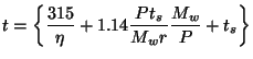 s (18)
The heating phase is controlled by the design parameters and includes the time required to heat the water that will eventually be lost due to evaporation. The simmer time depends on the type of food to cooked and is not governed by the stove design.
Some experimental results
The expression clearly demonstrates, that for a given quantity and type of food (that is, for a given Mw and ts , the well known experience that the specific fuel consumption decreases with efficiency. This was actually demonstrated by Dutt and Ravindranath (1993) by carrying out a typical cooking task with a wide variety of stoves. The cooking task prevalent in the village of Ungra in Southern Karnataka comprised of 1,102g of rice ( +2,121g of water), 883g of ragi flour a millet (+ 1,554g of water) 256g of cowpeas, a legume (+ 2,463g of water) and 150g of vegetables mixed with cowpeas. The result is shown in Fig.6. There is no doubt that there is a considerable scatter in data, but the trend in data clearly establish the fact that higher the water boiling test
Source: Dutt & Ravindranath (1993)
efficiencies lower the specific fuel consumption. However direct comparison between the calculated and measured fuel consumption figures is not feasible since the authors did not report power data.
A direct comparison between computed and measured fuel consumption values was carried out by Visser (1993) for cooking tests conducted in Senegal. The food and cooking scheme used in these tests are given below.
Quantities of food
| Oil | 660g |
| Tomato puree | 400g |
| fish | 1500g |
| Vegetables | 2000g |
| Rice | 2000g |
| Water | 2200g |
Power regime
- (i)
- Maximum power
Heating of oil to 200 °C
Heating of onions and tomato puree
Frying of onions and tomato puree
Heating of fish
Frying of fish
Heating of fish and vegetables
- (ii)
- Minimum power
Cooking of fish and vegetables - (iii)
- Average power
Steaming of rice - (iv)
- Minimum power
Cooking of rice.

Fig.7. Cooking experiment results from Senegal
Source:Piet Visser (1993)
The results of this work are presented as a set of bar charts in Fig.7.
Before leaving this question we need to look at another aspect which has to
do with the simmer time and its influence on fuel consumption. Eq.(17)
suggests that SFC increases linearly with simmer time as well as power
output (maximum) but inversely with
![]() ,
the turn down ratio. Fig.8 shows
the SFC for three hypothetical stoves as a function of simmer time. Stove 1
has the highest efficiency but a low turn-down ratio. Stove 2 has half the
,
the turn down ratio. Fig.8 shows
the SFC for three hypothetical stoves as a function of simmer time. Stove 1
has the highest efficiency but a low turn-down ratio. Stove 2 has half the
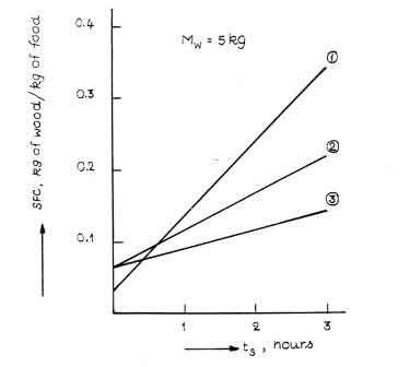
Fig.8. SFC as a function of simmer time
| 1 | 2 | 3 | |
| P, kW | 5 | 2.5 | 2.5 |
| r | 2 | 2 | 4 |
| n, % | 50 | 25 | 25 |
efficiency as well as half the power of stove 1. It is remarkable to note that except at very low simmer times (around half an hour) stove 2 outperforms stove 1 in spite of very low efficiency. Stove 3 is a handsome winner among the three contestants. This is a clear indication that high efficiency does not automatically guarantee a low specific fuel consumption. The latter is a strong function of the simmer time. In other words SFC is dependent on the task to be performed by the stove. Many recipes demand simmer times of the order of one hour or more. For such tasks it is essential for the stove to possess high turn-down ratio. However it is important to remember that there is a price to be paid if one were to choose stove 3 in the name of fuel economy. For a simmer time of 1 hour, stove 3 will finish the task in 1 hour and 45 minutes while stove 1 will need only one hour and 15 minutes. In particular if the simmer time is half hour or less the time difference will become sufficiently large for the cooks to start complaining about the stove taking too much time. Thus one needs to have a compromise. Before looking at the compromise, we shall look at the problem of obtaining reasonably high turn-down ratios with wood fires.
Simmer power
Simmering simply demands that the temperature of the pan contents be held at a given value, usually 100 ° C for cases where water is the cooking medium. This means that the fire has simply to supply the heat losses from the pan. A very thorough analysis of the problem was provided by Bussmann (1988). We have covered this in the page on Experiments.
Heat Balances
Introduction
Drawing a heat balance is an important diagnostic tool for determining the
most effective method of improving the performance of thermal equipment. It
is simply an accounting procedure to keep track of the way in which heat is
used and lost in the equipment concerned. The general idea of a heat balance
in a woodturning stove is depicted in Fig. 9. The diagram is an overall
representation of the processes in a stove. But we will concentrate on the
heat flows, the
![]() 's.
's.
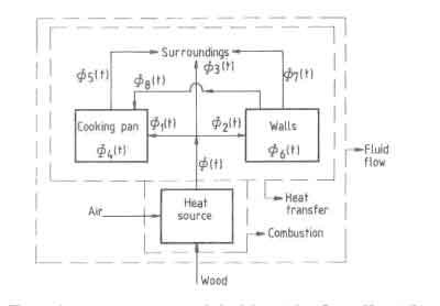
Heavy lines: system elements; light lines: interaction paths;
dashed lines: process identification
In principle, drawing a heat balance is the application of an energy equation. We have done this while calculating the fuelbed temperature and gas temperature resulting from the combustion of wood. In these attempts the time variable was completely ignored.
Drawing a serviceable heat balance is a demanding experimental chore. The reason one goes to this trouble, instead of stopping at a mere efficiency test, is the expectation that the heat balance will suggest promising avenues for plugging avoidable beat leaks in the system. An example will help in clarifying the nature of problems that can be solved by knowing heat balances. Consider the heat flows in the pan shield of a shielded fire. Figure 10 shows the different heat flows that occur in the system. The heat balance can be written as a function of the geometry, pan temperature, and shield properties. A relevant question is the effect of changing the shield properties, say, reducing its thermal conductivity by applying some form of lagging or inserting an insulating liner. If this procedure increases the efficiency of the device, it would be possible to estimate the trade-off between the cost of insulation and the increased efficiency. Of course, there will be the possibility of increased heat being carried away by the gases leaving the gap between the pan and the shield. In such a case the extra cost of insulating the shield may not be paid for by in- creased efficiency.
In the next section we will present a few examples of heat balances for several stoves before discussing the techniques of drawing heat balances.
Example Heat Balances
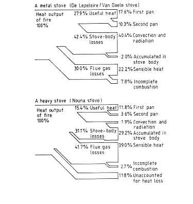
From time to time beat balances have been drawn for several types of woodburning cookstoves. Nievergeld et al. (1981) and Claus et al. (1981) carried out exhaustive measurements on a metal and a heavy stove, both of which use two pans. Two typical heat balances from these references are reproduced in Fig.11. The metal stove is obviously a better designed stove and has a much higher efficiency than the heavy stove. The other characteristic that emerges from a study of these heat balances is that the metal stove loses a lot of heat through its body. The heavy stove has much of its heat lost through the stack, though it has a better combustion efficiency. The main reason for this is that the stove drags in too much air. In addition, the stove has a rather poor arrangement of pan heat transfer surfaces. The closure of the heat balance in the heavy stove is also poorer. This is attributed to the difficulty in evaluating the heat accumulation in the stove body. In fact, Van der Heeden et al. (1983) show that by appropriately constricting the air supply, introducing a suitably designed baffle, and partially sinking the pans inside the stove body, the efficiency of the stove could be pushed up to 40% from 15%. This work was made possible only through a careful analysis of heat balances.
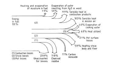
An interesting heat balance was provided by Geller in his study on cookstoves in south India (1983). Kitchen tests in this study were supplemented by laboratory studies. A typical heat balance emerging from this work is shown in Fig.12. Several differences between this and the previous figure need to be pointed out. Air-dried wood was used in the Geller work. As such, an additional item is introduced. A second difference arises in that the steam formation is treated as a loss (which is indeed true for the actual cooking process), while the work in Fig. 11 does not treat it so (a discussion on this point has already been given in the previous sections). A third feature is the remaining charcoal at the end of the cooking process. This charcoal is in principle recoverable and is to be used subsequently. Thus in terms of the results of Fig.11, the south Indian stove has an efficiency of 11.25%. As in the case of the heavy stove result of Claus et al., the unaccounted for heat loss is quite large-in fact it is the largest heat of account. It is clear that it is not easy to get closed heat balances in a woodstove.
to pan and environment
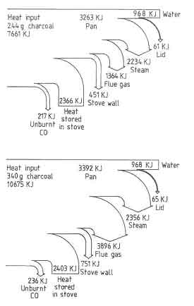
A final example of heat balance is from Dunn et al (1983) on a charcoal stove commonly used in Thailand. Two heat balances are shown in Fig. 13; one is for a restricted air supply and the other for a standard design. The figures clearly establish that an important method of increasing stove efficiency is to design a stove so that it draws just enough air for reason- ably complete combustion. Closed heat balances were obtained in this investigation principally because (1) charcoal was the fuel and (2) air flow through the stove was directly measured at the entry point.
These examples of beat balances show the many ways in which heat is lost in a stove. Improvement in stove efficiencies cannot be obtained by some magic formula (as is hoped for in many circles), but by patient work involving the plugging of various heat leaks.
Techniques of Estimating Heat Balances
We will now turn to a discussion of the techniques of drawing heat balances. Vermeer and Sielcken [74] provide a comprehensive list of items that account for the total amount of fuel used in a stove for a cooking scheme:
- 1. The pan:
- heating up the water and food;
- heat for chemical reactions during cooking;
- production of steam during the simmering period;
- heat stored in the pan; and
- heat lost due to convection and radiation from the pan walls.
- 2. The stove accounting for:
- (a) radiative and
- (b) convective heat losses of the exposed parts to the environment; and
- (c) the accumulated heat in the stove body.
- 3. Stack losses consisting of :
- (a) sensible heat carried away by the hot gases;
- (b) unburnt CO, and
- (c) unburnt CxH y.
- 4. Soot and tar deposits, partly stuck to the pan walls and the inside of the stove body and partly carried away by the flue gases.
- 5. Unburnt charcoal in the ash at the end of an experiment.
- 6. Loss of energy due to the presence of moisture in wood.
The examples in the previous section are overall heat balances and the checklist above also treats the subject in a similar manner. The measurements required, apart from those for an efficiency test, are temperatures at various positions on the stove body and the gas stream. In addition, a complete gas analysis is required. Since a stove rarely operates under steady-state conditions, all these quantities need to be recorded continuously throughout the experiment. This makes the problem of data handling and conversion of the data into a set of heat loss estimates quite a complicated enterprise.
Assuming that drawing a heat balance is the activity to be carried out in an engineering laboratory, we can postulate a well-designed experiment. Such an experiment will use oven-dry wood and will arrange to burn all the wood during the experiment. Thus items (5) and (6) do not enter the picture. Some experimental results (Nievergeld et al. 1981) suggest that soot, Cx H y, etc., do not add up to more than a couple of percentage points. The pan losses are quite small at least at the high power end of stove operation. Thus the discussion will be limited to three items: the absorption of energy by the pan contents, the stove body losses, and the stack losses. The first of these is evaluated in every efficiency test. Thus we need to look at two items. These two items will be discussed with reference to our prototypical example of the shielded fire, which has a relatively simple geometry- unlike the systems considered by Claus et al.(1981) and Geller (1983). In spite of these simplifications, drawing an acceptable heat balance is a formidable task.
Referring to Fig. 13, the heat loss from the stove surface could be split into three parts:
where i stands for combustion chamber or pan shield.
for the flat annular disk joining the combustion chamber and the pan shield. In the above expressions t, is the duration of the experiment; h is a fictitious heat transfer coefficient that clubs both radiation and convection heat losses.
In the above expression T can be measured in principle at any number of
points, subject to the number of available recording channels. How- ever,
evaluation of h(
![]() ,y,t) or h(
,y,t) or h(
![]() ,r,t) with the fire as the driving force is far too complex for such a
small device as a cookstove. There are four possible approximations one could use.
,r,t) with the fire as the driving force is far too complex for such a
small device as a cookstove. There are four possible approximations one could use.
- A temperature averaged over space and time with a free convection correlation for vertical surfaces.
- A temperature averaged over space, but evaluating heat loss for each interval of time again using a free convection correlation for vertical surfaces.
- A temperature averaged over the variables 0 and t along with free convection correlations for variable surface temperatures.
- A complete finite difference approximation-identifying an area around each measurement point-and heat loss evaluated from each surface element for small intervals of time using a relatively simple local heat transfer correlation.
The last approach is the one employed in the heat balance calculations of Nievergeld et al. (1981) and Claus et al. (1981)
The next item is the evaluation of heat carried away by the combustion gases leaving the top of the shield-pan gap.
Air/gas flow measurement is one of the most difficult assays to accomplish for the small devices operating on natural draft. Direct measurement of air flow at an inlet, as used by Dunn et al. (1983), is difficult for a device of the type shown in Fig. 13, for which air admission occurs through a series of holes arranged around the periphery of the fire box below and above the grate. Measurement of velocity in the shield-pan gap is difficult due to the rather low velocities, high temperatures, and unclean nature of the gas. Thus mass flows are essentially inferred by:
- gas analysis;
- amount of wood burned;
- ultimate analysis of wood; and
- appropriate stoichiometric relations. All the problems connected with averaging mentioned in connection with temperature measurement exist for gas analysis as well. The situation for chimney stoves is somewhat simpler than for devices of the type shown in Fig. 10.
Summarizing, to obtain a closed heat balance within about 10% for a stove for the experimental duration is an ambitious undertaking and is probably not called for in most circumstances.
For steady periodic operation of a chimney stove (if it can be realized), the method used by Pessers (1983) may prove useful. He inferred the instantaneous mass flow through the chimney by equating the heat loss from a certain portion of the chimney to the sensible heat loss of the gas flowing over the same portion. His technique produces mass flow results that are within 5% of those obtained by the carbon-balance technique. This suggests that the latter is quite satisfactory for most cases. Vermeer and Sielcken (1983) provide a detailed analysis of the procedure. The method of Pessers combined with continuous monitoring of fuel- and water-weight loss will provide a means of drawing heat balances as a function of time for the duration of operation of the stove.