home
needs
local resources
comfort
safety & health
contact
reports
Heat transfer
- Open Fire: Characteristics Of Heat Transfer To A Pan
- Radiation from the Fuelbed
- Radiation from the Flames
- Emission of the soot particles
- Emissivity of the gases
- The total emissivity of the flames
- Convective Heat Transfer to the Pan
- Flow field
- Temperature
- Heat transfer Coefficients
- Results and discussion
Radiation from the Fuelbed
According to Fig.4.10, it can be stated that the temperature of the fuelbed is about 900 K when the excess-air factor is between 1 and 2. In order to calculate the radiative energy transfer from the fuelbed to the pan, we assume that the gases and flames between the pan and fuelbed do not absorb or emit any radiation. The view factor F between fuelbed and pan is equal to the view factor of two concentric parallel disks and can be found in many textbooks (see, for example, Sparrow and Cess 1970).
In order to check the estimated temperatures of the fuelbed and thus the radiative hat transfer to the pan, experiments were done by Herwijn with a radiative heat flux meter above a woodfire. The estimates of the fuelbed temperatures and the measured temperatures are presented in Table 5.1. The experimental results are obtained for a fire on a grate. The power density of the fire is 18 W/cm". In order to simulate a steady fire, the wood is added in small blocks. With such a procedure almost no distinction can be made between the burning of volatiles and charcoal. The temperatures are calculated from the measurements according to the following formula:
| (1) |
Here ![]() is the total radiosity arriving at the instrument.
is the total radiosity arriving at the instrument. ![]() the fuelbed surface,
the fuelbed surface, ![]() the view factor from fuelbed to the radiation
meter,
the view factor from fuelbed to the radiation
meter, ![]() the temperature of the fuelbed, and
the temperature of the fuelbed, and ![]() the temperature of
the radiation meter. The estimated temperatures are calculated according to
Eq.(4.15); for these calculations the excess air factor
the temperature of
the radiation meter. The estimated temperatures are calculated according to
Eq.(4.15); for these calculations the excess air factor ![]() is taken
to be 1. The differences in the estimated temperatures are due to the
variation of the power density on the grate.
is taken
to be 1. The differences in the estimated temperatures are due to the
variation of the power density on the grate.
In general, the measurements and estimated temperatures compare well. Although the measured temperatures with eccentric displacement of the meter are lower compared to the temperatures with a concentric situation, the deviation is within 15%.
| Sl. No. |
P (kW) |
b (cm) |
H (cm) |
e (cm) |
G |
||
| Measured | Estimated | ||||||
| 1. | 3.5 | 18 | 15 | 0 | 10 | 910 | 880 |
| 2. | 5.9 | 20 | 15 | 0 | 15 | 960 | 950 |
| 3. | 7.0 | 22.5 | 15 | 0 | 19 | 985 | 940 |
| 4. | 8.8 | 25 | 15 | 0 | 23 | 995 | 940 |
| 5. | 5.9 | 20 | 10 | 0 | 21 | 930 | 950 |
| 6. | 5.9 | 20 | 10 | 8 | 7.1 | 775 | 950 |
| 7. | 5.9 | 20 | 15 | 8 | 7.8 | 880 | 950 |
| 8. | 8.8 | 25 | 15 | 8 | 8.7 | 900 | 940 |
Using the above information we obtain the results for the radiant heat
transfer to the whole pan as shown in Table 2. The calculations are based
on a pan of 100 ° and the measured fuelbed temperatures
calculated form Eq.(1). The view factor is taken for a pan of 28-cm
diameter placed 15 cm above the fuelbed. The diameter of the fuelbed varies
with the power of the fire such that the power density is constant at 18
![]() . From the table it appears that 12% of the wood heat is
radiated to the pan.
. From the table it appears that 12% of the wood heat is
radiated to the pan.
| Sl. No. |
P (kW) |
Tb (K) |
|||
| (kW) | (%) | ||||
| 1. | 3.5 | 910 | 0.42 | 0.41 | 11.7 |
| 2. | 5.9 | 960 | 0.41 | 0.62 | 10.5 |
| 3. | 7.0 | 985 | 0.39 | 0.82 | 11.8 |
| 4. | 8.8 | 995 | 0.38 | 1.04 | 11.8 |
If we compare this to the efficiency achieved through common practice in developing countries - an open-fire efficiency between 10 and 15% - it can be stated improved stoves can only show a higher efficiency due to optimal use of the convective heat transfer.
Radiation from the Flames
One of the factors that determines the radiation from the flames is the emissivity. The total emissivity of the flames is a superposition of the contribution from the soot particles and the gases.
Emission of the soot particles
The emissivity of the soot particles is dependent on two quantities, the
flame height and the volume fraction of the soot particles in the flames.
When using an open fire, it is common observation that soot will deposit on
the cold pan. From experiments it appears that on the average about 5 g of
soot deposits on the pan when burning 1 kg of wood. With an excess-air
factor 3 we find a volume fraction for the soot particles of about 2.10![]() . This agrees reasonably well with experiments done in a closed brick
stove, where a soot concentration between 5 and 10
. This agrees reasonably well with experiments done in a closed brick
stove, where a soot concentration between 5 and 10
![]() of
the combustion products was found (Claus et al. 1981).
of
the combustion products was found (Claus et al. 1981).
Using the work of Felske and Tien (1973) to calculate the emissivity of the soot we find a value between 0.025 and 0.036 for a fire power between 3 and 8 kW.
Emissivity of the gases
Of the gases commonly present in a fire, only
![]() and
and
![]() contribute to the emissivity. The other gases (
contribute to the emissivity. The other gases (
![]() and
and
![]() ) consist of symmetrical molecules that emit and absorb
radiation only at much higher temperatures. In order to make an estimate of
the emissivity of the gases
) consist of symmetrical molecules that emit and absorb
radiation only at much higher temperatures. In order to make an estimate of
the emissivity of the gases
![]() and
and
![]() we will
assume that no incomplete combustion will occur and that the total
excess-air factor is equal to 2.
we will
assume that no incomplete combustion will occur and that the total
excess-air factor is equal to 2.
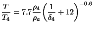
Hottel (1954) presents graphs from which the emissivity of the carbon
dioxide and the water vapor can be determined. Hottel also gives a method to
determine the mean beam length, depending on the volume, to be used with the
graphs. For our calculations we assume that the reference volume is a
circular cylinder with a radius equal to the radius of the flames at their
tips. The emissivity for the total gas radiation is listed in Table 3 as a
function of the power of the fire. In this table also the emissivity of the
soot particles is given.
| P (kW) |
h (cm) |
(cm) |
(m2) |
(W) |
(%) |
|||
| 1 | 8 | 25 | 0.016 | 0.035 | 0.050 | 0.016 | 61 | 6.1 |
| 2. | 10.5 | 3.2 | 0.021 | 0.041 | 0.061 | 0.028 | 128 | 6.4 |
| 3. | 12.3 | 3.8 | 0.025 | 0.045 | 0.069 | 0.038 | 200 | 6.7 |
| 4. | 13.8 | 4.3 | 0.028 | 0.049 | 0.076 | 0.049 | 280 | 7.0 |
| 5. | 15.1 | 4.7 | 0.031 | 0.051 | 0.080 | 0.059 | 348 | 7.0 |
| 6. | 16.2 | 5.0 | 0.032 | 0.053 | 0.083 | 0.067 | 417 | 6.9 |
| 7. | 17.2 | 5.4 | 0.035 | 0.055 | 0.088 | 0.076 | 503 | 7.2 |
| 8. | 18.2 | 5.6 | 0.036 | 0.057 | 0.091 | 0.084 | 575 | 7.2 |
| 9. | 19.0 | 5.9 | 0.038 | 0.059 | 0.095 | 0.092 | 659 | 7.3 |
| 10. | 19.8 | 6.1 | 0.039 | 0.060 | 0.097 | 0.099 | 724 | 7.2 |
The total emissivity of the flames
In order to calculate the total emissivity of the flames one has to
determine the effect of mutual absorption of the radiation from the gases
and soot. Tien et al. (1972) give a simple formula to calculate the total
emissivity
![]() when both soot emissivity
when both soot emissivity
![]() and gas
emissivity
and gas
emissivity
![]() are known. This formula is
are known. This formula is
| (2) |
In Table 3 the total emissivity is listed; also the total luminous
radiative power ![]() is given. We see that the flame radiation is
about 7% of the total power of the fire. For these calculations an
excess-air factor for the volatiles is taken to be 3. According to Fig.1
the average gas temperature for this situation is about 1400 K. Now that we
know the part of the power of the fire that is converted to the radiation of
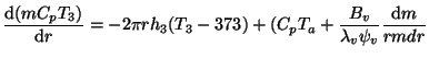
the flames, we can revise the solution of Eq. (5.17). This is approximated
by
is given. We see that the flame radiation is
about 7% of the total power of the fire. For these calculations an
excess-air factor for the volatiles is taken to be 3. According to Fig.1
the average gas temperature for this situation is about 1400 K. Now that we
know the part of the power of the fire that is converted to the radiation of
the flames, we can revise the solution of Eq. (5.17). This is approximated
by
where ![]() and
and ![]() are the mass flow and the combustion value of the
wood respectively. The temperature of the gases becomes lower due to this
correction. The result is given in Fig.1. The (small) decrease in
temperature of the gases does not influence the emissivity factors listed in
Table 3.
are the mass flow and the combustion value of the
wood respectively. The temperature of the gases becomes lower due to this
correction. The result is given in Fig.1. The (small) decrease in
temperature of the gases does not influence the emissivity factors listed in
Table 3.
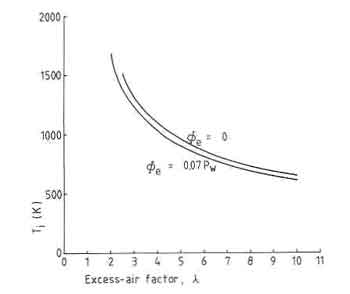
Fig.1. Gas temperatures for losses due to the radiation from flames
In experimental work the part of the flame radiation detected by the
radiative heat flux meter has to be estimated in order to check whether a
correction should be applied for this contribution. For this correction we
consider the source of the flame radiation to be circular, with equal power
in the total column and the same diameter. This source is placed in the
middle between fuelbed and meter. The part of the flame radiation impinging
on the radiation meter is determined by the view factor. Because this view
factor is for the given situation, of the order of 10![]() , no correction
is needed for the temperatures of the fuelbed.
, no correction
is needed for the temperatures of the fuelbed.
The contribution of the flame radiation to the heat transfer to the pan can be estimated in the same way. In this situation the view factor is 0.4, which means that due to flame radiation 3% of the total power impinges on the pan bottom.
Convective Heat Transfer to the Pan
Three factors determine the convective heat transfer to the pan on an open fire in a wind-free environment:
- (i)
- power level of the fire;
- (ii)
- the height between the fuelbed top and pan bottom; and
- (iii
- the pan-fuelbed geometry.
The efficiency of the heat transfer process can be defined in terms of ![]() , the exit temperature of the combustion gases (the average gas
temperature at the top plane of the pan), and
, the exit temperature of the combustion gases (the average gas
temperature at the top plane of the pan), and ![]() , the pan temperature.
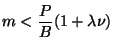
When
, the pan temperature.
When
![]() , heat is carried away unutilized and when
, heat is carried away unutilized and when
![]() ,
the pan loses heat. A loss in efficiency is the result in either case.
Figure depicts six hypothetical cases schematically corresponding to the
three factors mentioned above. For a well-matched power level of the fire,
the height of the pan above the fuelbed and the pan geometry
,
the pan loses heat. A loss in efficiency is the result in either case.
Figure depicts six hypothetical cases schematically corresponding to the
three factors mentioned above. For a well-matched power level of the fire,
the height of the pan above the fuelbed and the pan geometry ![]() will be
within a few degrees of
will be
within a few degrees of ![]() .
.
Fig.2. Among power level, distance between pan bottom and fuel bed and pan geometry
In order to make an estimate of the convective heat transfer from the hot
gases to the pan one has to know the temperature of the combustion gases as
well as the convective heat transfer coefficient. In general, the convective
heat transfer ![]() is given by the relation
is given by the relation
| (3) |
where ![]() is the heat transfer coefficient,
is the heat transfer coefficient, ![]() the concerned surface, and
the concerned surface, and ![]() and
and ![]() the gas and pan temperature, respectively. Before we present
estimates of temperature and heat transfer coefficients we first divide the
area around the pan into several subregions, each with its own flow
characteristic and a general method to estimate the gas temperature.
the gas and pan temperature, respectively. Before we present
estimates of temperature and heat transfer coefficients we first divide the
area around the pan into several subregions, each with its own flow
characteristic and a general method to estimate the gas temperature.
When we observe an impinging jet on a flat plate held normal to the jet, we
see a stagnation point region along the line of symmetry where the boundary
layer is expected to have constant thickness. Of course, this may not be
true in the presence of combustion. Beyond this region, over the outer half
of the pan bottom, the flow could be treated as an axisymmetric wall jet. At
the pan corner the gases turn again over an angle of ![]() due to the
buoyancy forces and will rise up along the pan wall. Figure 3 shows the
several regions; the bending of the flow around the corner of the bottom is
treated as a separate region and the flow along the pan wall is divided into
regions where combustion occurs and where no combustion occurs. For each
region a heat balance can be made. It will have the general form
due to the
buoyancy forces and will rise up along the pan wall. Figure 3 shows the
several regions; the bending of the flow around the corner of the bottom is
treated as a separate region and the flow along the pan wall is divided into
regions where combustion occurs and where no combustion occurs. For each
region a heat balance can be made. It will have the general form
| (4) |
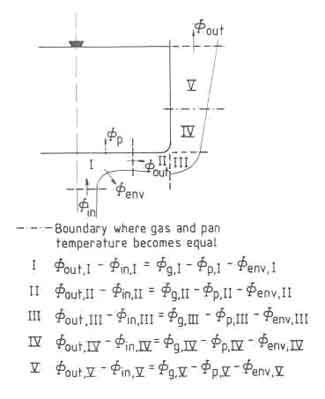
Fig.3. es under and along a pan for which a heat balance has to be drawn
| I. |
|
|
|
| II. |
|
|
|
| III. |
|
|
|
| IV. |
|
|
|
| V. |
|
|
|
In words this means that the difference in energy content of the gas leaving
a region (
![]() ) and entering a region (
) and entering a region (
![]() ) is balanced by
the heat production due to combustion (
) is balanced by
the heat production due to combustion (
![]() ) minus losses to the pan
(
) minus losses to the pan
(
![]() ) and losses to the environment (
) and losses to the environment (
![]() ) whether due to
radiation or due to dilution by entrainment of air. In general, the
combustion stops in region IV, which means that in region IV the
contribution of
) whether due to
radiation or due to dilution by entrainment of air. In general, the
combustion stops in region IV, which means that in region IV the
contribution of
![]() is zero. In region III the heat losses to the
pan can be assumed zero because the pan surface exposed here is negligible.
The inlet temperature of each region is of course equal to the outlet
temperature of the previous region. As of now such a calculation, which
requires a complete numerical scheme, has never been attempted. There have
been several attempts to provide approximate results for the heat transfer
to the pan. The first one was due to Krishna Prasad et al. (1985) and a much
more refined version was provided by Bussmann (1988). We shall describe the
latter work in detail.
is zero. In region III the heat losses to the
pan can be assumed zero because the pan surface exposed here is negligible.
The inlet temperature of each region is of course equal to the outlet
temperature of the previous region. As of now such a calculation, which
requires a complete numerical scheme, has never been attempted. There have
been several attempts to provide approximate results for the heat transfer
to the pan. The first one was due to Krishna Prasad et al. (1985) and a much
more refined version was provided by Bussmann (1988). We shall describe the
latter work in detail.
Flow field
A schematic view of the fuelbed-flame-pan configuration is shown in Fig. 4 . The figure indicates the four regions of interest;
- a jet formed by the flame (1);
- the stagnation point flow region formed by the jet impinging on the pan bottom (2);
- the axisymmetric wall jet region formed along the pan bottom by the
gases turning by an angle of
 /2 radians (3); and
- finally a two-dimensional wall-jet region along the pan wall (4).
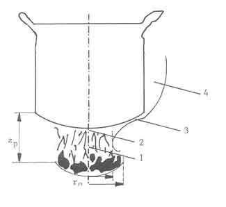
Fig.4. w of fuelbed-flame-pan configuration
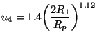
Available literature on modelling flow characteristics of impinging jets
uses the diameter of the nozzle exit (![]() ) as the characteristic
length. For woodfires the value of
) as the characteristic
length. For woodfires the value of ![]() is chosen to be the diameter of
the hot gas plume at the top of the flame. However when the distance between
the pan and the fuelbed (
is chosen to be the diameter of
the hot gas plume at the top of the flame. However when the distance between
the pan and the fuelbed (![]() ) is smaller than the flame height,
) is smaller than the flame height, ![]() is set equal to the calculated diameter of the fire at the pan height.
is set equal to the calculated diameter of the fire at the pan height.
Bussmann assumed that the stagnation point flow regime covers
| (5) |
In this region it is also assumed that no ambient air is entrained. This
assumption is based on the work of Era and Saima (1976) who investigated the
flow characteristics of an axisymmetric wall jet created by gases issuing
from a nozzle and impinging on a flat plate held close to the nozzle tip. In
the axisymmetric wall region there is an increase in the mass flow rate due
to entrainment of air from the ambient and is estimated from the
semi-empirical relation (Hertel 1962)
| (6) | |||
| (7) |
The flow field at the pan corner is difficult to describe. Thus Bussmann assumed that no air entrains at the corner and the flow develops into a two-dimensional wall jet as soon as it comes into contact with the pan side.
Temperature
The next step in the model is to estimate the temperatures prevailing in the different flow regions described above. The stagnation point region is divided into two regions.
(i)
![]()
![]() is the temperature at the pan height calculated from the flame model
presented in 5.2. According to this model
is the temperature at the pan height calculated from the flame model
presented in 5.2. According to this model ![]() is not a function of
is not a function of ![]() and thus is constant.
and thus is constant.
(ii)
![]()
The temperature in this region is evaluated from a simple heat balance
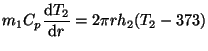 |
(8) |
The heat balance provides temperature as a function of radius and accounts
for heat loss from the gas stream to the pan. ![]() is the heat transfer
coefficient in this region.
is the heat transfer
coefficient in this region.
The temperature in the axial wall jet region
![]() , where
, where ![]() is the radius of the pan, is obtained from the quasi-empirical relation
provided by Hertel (Eq.5.21) and the following heat balance equation.
is the radius of the pan, is obtained from the quasi-empirical relation
provided by Hertel (Eq.5.21) and the following heat balance equation.
 |
(9) |
The first term on the right represents the heat absorbed by the pan. The second term comes in two parts both associated with the entrainment of outside air. The first part simply accounts for the heat content of the entrained gases. The second part accounts for the heat liberation by combustion. Note that this term was absent in the stagnation point region. This is primarily due to the manner in which the flame model was implemented. That model is always computed on the basis of a chosen amount of excess air factor at every height. Since there is no additional air entrained in the stagnation region our flame model will not yield any heat release. The inclusion of heat release in this region is also questionable in the sense it is outside the calculation possibility of our flame model since it is only one-dimensional (that is, heat release occurs only as a function of height in the flame model; in the region below the pan the height is constant). Thus both cases - with and without combustion - was investigated by Bussmann. There is yet another consideration - volatiles coming out of the fuel bed should not all have been consumed before the gases arrive at the pan. Thus
 |
(10) |
![]() here represents the volatile fraction and
here represents the volatile fraction and ![]() is the excess air
factor. The last zone where temperature has to be estimated is in region 4
mentioned earlier. Bussmann assumed that the thickness of the hot gas layer
along the vertical side of the pan to be small in comparison to the radius
of the pan. This assumption permits the use of a relation proposed by Seban
and Back (1961) for a two-dimensional wall jet
is the excess air
factor. The last zone where temperature has to be estimated is in region 4
mentioned earlier. Bussmann assumed that the thickness of the hot gas layer
along the vertical side of the pan to be small in comparison to the radius
of the pan. This assumption permits the use of a relation proposed by Seban
and Back (1961) for a two-dimensional wall jet
 |
(11) |
![]() in the above is taken as the temperature at the bottom corner of the
pan and is consistent with the assumption that there is no air entrained in
the corner. This probably will lead to an overestimate of
in the above is taken as the temperature at the bottom corner of the
pan and is consistent with the assumption that there is no air entrained in
the corner. This probably will lead to an overestimate of ![]() .
. ![]() ,
the thickness of the wall jet at the bottom corner, is calculated from
,
the thickness of the wall jet at the bottom corner, is calculated from
| (12) |
where ![]() is taken to be the velocity at the pan bottom corner. From the
work of Era and Saima, cited earlier, we obtain for
is taken to be the velocity at the pan bottom corner. From the
work of Era and Saima, cited earlier, we obtain for ![]() the following
relation.
the following
relation.
 |
(13) |
Heat transfer Coefficients
In order to evaluate the various temperatures above and to estimate the total heat transfer to the pan, we need to know the heat transfer coefficients. These are the same as the ones used in Bussmann et al (1983) and reproduced here.
- (i) For the stagnation point region the Nusselt number relationship
proposed by Schlunder and Gnielinski (1976) is used.
 (14)
(14)
 denotes the average heat transfer coefficient.
- (ii) For the axisymmetric wall jet, the relation proposed by Hrycak
(1978) is used.
 (15)
(15)
Re in Eqs. (5.29) and (5.30) is based on the length
 .
.
- (iii) For the pan side the relationship given by Seban and
Back(1961) is used.
 (16)
(16)Re here is based on the length, l, the distance along the pan side from the pan bottom.
Results and discussion
We will now present the results obtained from the above analysis. Fig. 5 presents the results of gas temperatures under the pan as a function of the radial distance.The three pairs of solid and dashed curves correspond to temperatures obtained for three distances between fuelbed and pan bottom - 0.1, 0.15 and 0.2m.
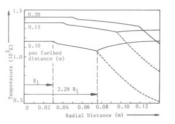
Fig.5. Distribution in the gas under the pan for different pan-fuelbed disaxial wall jet without combustion in axial wall jet
The pan radius for these calculations is 0.14m. The solid and dotted lines
denote respectively the cases with and without combustion being considered
in the axial wall jet. The discontinuity at ![]() is due to the fact
that a correction has been incorporated for heat absorption in the central
region of the pan bottom. The discontinuity at
is due to the fact
that a correction has been incorporated for heat absorption in the central
region of the pan bottom. The discontinuity at
![]() is due to the
fact that the axial wall jet relationship is applicable from this point
onwards. The result for the largest distance shows that there is no
combustion along the pan bottom at all due to the fact the volatiles have
been exhausted by the time the gases arrive at the pan bottom. Furthermore
at the lowest distance, the temperature at the bottom corner of the pan
drops to 500K in the absence of combustion. This is unrealistic. At this
height, even if we include combustion the temperatures at the bottom corner
does not even reach the values at the axis for the largest distance. Thus
considerable amount of combustion is likely to occur on the side of the pan.
According to our heuristic discussion in connection with Fig.2 this is
undesirable.
is due to the
fact that the axial wall jet relationship is applicable from this point
onwards. The result for the largest distance shows that there is no
combustion along the pan bottom at all due to the fact the volatiles have
been exhausted by the time the gases arrive at the pan bottom. Furthermore
at the lowest distance, the temperature at the bottom corner of the pan
drops to 500K in the absence of combustion. This is unrealistic. At this
height, even if we include combustion the temperatures at the bottom corner
does not even reach the values at the axis for the largest distance. Thus
considerable amount of combustion is likely to occur on the side of the pan.
According to our heuristic discussion in connection with Fig.2 this is
undesirable.
Figure 6 presents the average heat transfer coefficients over the entire pan as a function of pan-grate distance. These were computed on the basis of an average temperature difference between the gas and the pan. The figure shows an increasing heat transfer coefficient with increasing pan-grate distance. The experimental results of Herwijn on the contrary show a rather constant value. The difference must be attributed to the conditions for which the relations (5.28) - (5.30) were derived. For example the Schlunder - Gnielinski formula was derived for a turbulent jet with a distance between the nozzle and the plate being between the nozzle diameter and 12 times the value. The Reynolds numbers in the fires of interest here can be much smaller and the flow is probably not laminar but cannot be fully developed turbulent either.
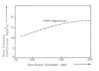
fig. 6. Coefficient at the pan bottom as a function pan to fuelbed distance.
What is more the distance between the grate and pan bottom corresponds to the lower end of the limit prescribed by Schlunder and Gnielinski. Thus in calculating efficiencies a constant value of the heat transfer coefficient is adopted, but it will be varied parametrically.
The next three figures (7 - 10) show some of the more significant
results obtained from the heat transfer calculation procedure presented
above. Fig.7 presents efficiency as a function of the pan-fuelbed
distance for three values of heat transfer coefficients, namely, 5, 10 and
15
![]() .
The flame parameters used in these calculations are:
the excess air factor
.
The flame parameters used in these calculations are:
the excess air factor
![]() ; the entrainment constant,
; the entrainment constant,
![]() ; and volatiles fraction,
; and volatiles fraction, ![]() . The fuelbed diameter is held
constant at 0.18m, the pan diameter is 0.28m and the combustion value of
wood is taken to be 18.7MJ/kg.
. The fuelbed diameter is held
constant at 0.18m, the pan diameter is 0.28m and the combustion value of
wood is taken to be 18.7MJ/kg.
The solid lines give the efficiencies obtained by including combustion in
the axial wall jet region while the dotted line shows the result without
combustion for the case with heat transfer coefficient of
![]() . The calculations incorporate corrections for the fuelbed thickness and the
so-called averaged peak power of the volatiles. The nature of these concepts
are discussed in connection with the experimental results to be presented in
the next section. The figure also shows the comparison of the theory with
experiment. It is easy to see the excellent agreement between theory and
experiment when one uses a heat transfer coefficient of 10W/m"K. In addition
it is also seen that it is important to account for the combustion in the
axi-symmetric wall jet region under the pan. This result confirms our
comment earlier on this question.
. The calculations incorporate corrections for the fuelbed thickness and the
so-called averaged peak power of the volatiles. The nature of these concepts
are discussed in connection with the experimental results to be presented in
the next section. The figure also shows the comparison of the theory with
experiment. It is easy to see the excellent agreement between theory and
experiment when one uses a heat transfer coefficient of 10W/m"K. In addition
it is also seen that it is important to account for the combustion in the
axi-symmetric wall jet region under the pan. This result confirms our
comment earlier on this question.
The next figure (Fig.8) compares the efficiencies obtained from
experiments carried out with different wood species and the theoretical
results. In the experiments the nominal power for definition;
also the next section) was held constant.
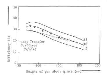
Fig.7.A function of pan-fuelbed distance. The points are from experiment the dotted line is without combustion for h = 10W/m2K.
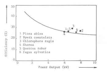
Fig.8.a function of the power of the fire. Points are experimental results with different wood species.
However corrections have been introduced in the calculated efficiencies for the measured differences in the averaged peak power. For this reason the results are shown in terms of power output. The calculations have all been performed by assuming a uniform fuelbed thickness of 50mm. It is seen that calculated values are in good agreement with the experiments. The somewhat larger deviations from theory seen for species 2 and 3 must be attributed to the inevitable variations in the fuel bed thickness in the experiments (see next section).
Finally Fig.9 shows a break-up of efficiency in terms of heat transfer by radiation and convection as reported by Krishna Prasad et al. (1985). The convective heat transfer is further divided into heat transfer to the bottom of the pan and the pan side. The heat transfer to the pan bottom above an open fire was measured with a heat flow meter by Herwijn (1984). This meter was placed such that the detecting surface lies in the plane of the pan bottom. The heat flow meter measures the radiant as well as the convective heat flux to the surface. Tests were performed for two powers of the fire, 6 and 8.7 kW; two distances between pan and fuelbed, 10 and 15 cm; and two eccentricities of the heat flow meter in the pan, 0 and 8 cm (the pan was always placed concentric with the fire). Table 5.4 gives a more detailed presentation of the measurements. The radiative contribution to the heat transfer found earlier can be subtracted from the total measured heat transfer. This gives an estimate of the convective heat transfer. These values are also listed in the table. The total, radiative, and convective heat transfer are related to the power of the fire in order to get the efficiency contribution of the various terms. The efficiency obtained for the convective contribution is obtained as before by dividing the pan bottom into two regions: the stagnation point region and the axisymmetric wall jet region. The radius of the boundary between the two regions is taken to be equal to the plume diameter calculated in the flame height model.
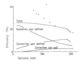
Fig.9. Efficiencies according to heat transfer by radiation and convection. Points are from experiments of Herwijn (1984)
In Fig. 9 the estimated efficiencies for a 6-kW fire are shown. Although
the measured radiative contribution agrees well with the model, as already
was shown in Table 2, the convective contribution to the pan bottom does
not agree at all. The main reason for this disagreement is the assumption
that the combustion stops at the pan height. This has been corrected in the
work of Bussmann.
| Sl. No. |
P (kW) |
(cm) |
(cm) |
(cm) |
(kW/m2) |
(kW/m2) |
(kW/m2) |
| 1. | 6.0 | 15 | 20 | 0 | 32.4 | 17.5 | 14.9 |
| 2. | 5.8 | 15 | 20 | 8 | 25.8 | 17.9 | 7.9 |
| 3. | 8.8 | 15 | 25 | 0 | 37.1 | 14.4 | 22.8 |
| 4. | 8.6 | 15 | 25 | 8 | 28.2 | 19.5 | 8.7 |
| 5. | 5.9 | 10 | 20 | 0 | 37.9 | 21.0 | 16.9 |
| 6. | 6.0 | 10 | 20 | 8 | 32.5 | 25.5 | 7.0 |
The point about this earlier work is it clearly establishes the relative importance of radiative and convective heat transfer to the pan. At the low height the radiative heat transfer contributes as much as one-third of the total heat input to the pan. At larger heights the importance of radiation goes down, A second point of importance that emerges from this figure is the fact that the convective heat transfer to the bottom and side of the pan are of equal orders of magnitude. Thus many a multi-pan improved stove with a chimney do not provide for heat transfer to the pan sides. Of course they do provide additional heat transfer surface by adding more pans. But that makes the stove bulky. Hence it is important to clearly delineate the merits of such stoves in comparison to single pan stoves that provide for adequate heat transfer surface.
total stove system