Flame Heights and Temperature Profiles
In this section we will review in detail the available theoretical and experimental evidence on the characteristics of the flaming combustion zone. As pointed out in the previous section. it is cumbersome to solve the general equations governing the processes in this zone. In particular, the outcome of such an exercise is uncertain because of difficulties in adequately accounting for radiation and turbulence. Therefore it is preferable to work with simpler models that can be validated by carefully designed experiments. Experiments also pose a severe problem in the sense that a wood fire is a hostile environment to carry out reliable and prolonged measurements. There is, however, one quantity that can be easily measured - the flame height. The starting point for the model is the work of Lee and Emmons (1961). They considered a turbulent plume above a steady two-dimensional source of hot fluid in a uniform stationary ambient environment. The equations of motion and energy were solved approximately to obtain analytical expressions for plume width, the buoyancy force and gas velocities as a function of height above the source. A similar model was developed by Steward (1970) for circular fires taking into account the liberation of heat by combustion in the first part of the hot gas column. This was done by assuming that combustion will provide a heat source in the equation. Such an approach has many advantages compared to the formulations in the previous sections. It treats the process of pyrolysis as simply the provider of a combustible gas to the flame zone. It ignores the details of the chemistry of combustion in the flame zone. Thus the species continuity equation (Eq.4.28) is replaced by a global conservation of mass equation. By the same token the reaction rate equation (Eq.4.31) is also ignored. This creates enormous simplifications for the model. For solving the problem Steward rewrote the continuity equation to provide the amount of air entrained at a given height above the fuelbed. The model thus predicts exclusively the flame heights. The mathematical simulation provided results that were in agreement with the experimental data if the excess air factor is about 4. It is thus believed that a model of the type of Steward will provide acceptable results for different classes of fires according to Cox and Chitty (1980).
For application to woodstoves the flame height is alone insufficient. We
have to know information about velocities and temperatures in order to
predict the heat transfer to the pan. Thus Bussmann et al. (1983; see also
Bussmann 1988) handled the continuity equation in a manner similar to the
one proposed by Lee and Emmons. The problem is treated as a turbulent free
convection problem. The geometry of the axisymmetric buoyant plume with
combustion is shown in fig.1. The entrained air is assumed to react
instantaneously with unburned fuel to stoichiometric completion. This avoids
the complexities of chemical reaction. The latter just provides a known
source term in the energy equation.
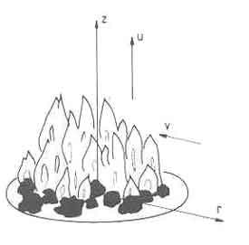
Fig.1. Geometry and coordinate system for an axisymmetric plume with combustion
The opportunity was used to review the entrainment information in more recent literature and appropriate modification to Steward's theory was introduced. Since this work is used in the next section for deriving heat transfer estimates, we will present some details about it. The governing equations are written in the integral form instead of differential form (See Schlichting, 1979, for derivation of these equations) for an axisymmetric buoyant plume with combustion. The volatiles, the combustion gases, and the entrained air are assumed to possess the same properties (independent of temperature), the same molecular weight and to obey the perfect gas equation of state. The pressure is taken to be uniform everywhere. The entrainment assumption of List and Imberger (1973) is used.
 |
(1) |
where ![]() , the entrainment constant, is taken as 0.08, which is considered
suitable for buoyant plumes. Steward used a value of 0.057, which is the
constant for round jets. The source term in the energy equation is given by
, the entrainment constant, is taken as 0.08, which is considered
suitable for buoyant plumes. Steward used a value of 0.057, which is the
constant for round jets. The source term in the energy equation is given by
 |
(2) |
The dimensionless forms of the integrated equations simplify to two
equations for the dimensionless momentum flow rate and dimensionless
density. The dimensionless quantities are defined by
| (3) | |||
 |
(4) | ||
 |
(5) | ||
| (6) | |||
| (7) |
The governing equations then are
Momentum:
 |
(8) |
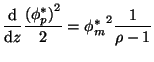
Energy:
![$\displaystyle {\frac{\mathrm{d}}{\mathrm{d}z}}{\frac{\phi _{m}^{\ast }}{\rho }}...
...rac{<tex2html_comment_mark>11 \mathrm{d}}{\mathrm{d}z}}[(1+v)\phi _{m}^{\ast }]$](flameheight/img15.png) |
(9) |
In these equations
![]() is uniquely determined from the mass
flow rate issuing out of the fuelbed and entrained air flow at any point.
Equations (5.3) and (5.4) are solved easily for
is uniquely determined from the mass
flow rate issuing out of the fuelbed and entrained air flow at any point.
Equations (5.3) and (5.4) are solved easily for ![]() and
and
![]() to yield
to yield
![]()
![]()
The other physical variables can then be easily evaluated.
The plume geometry is given by
 |
(10) | ||
 |
(11) |
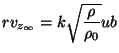
The local velocity is
| (12) |
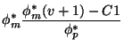
The integration constants C![]() and C
and C![]() are given by
are given by
![$\displaystyle \rho _{0}^{\ast }\mathrm{Fr}\left[ v-{\frac{1-\rho _{0}^{\ast }}{%%
\rho _{0}^{\ast }}}\right]$](flameheight/img30.png) |
(13) | ||
| (14) |
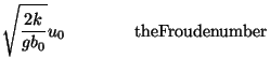
In order to relate the above results to combustion practice, ![]() in the
Froude number is written in terms of the rate of liberation of volatiles and
the fuelbed geometry. Thus
in the
Froude number is written in terms of the rate of liberation of volatiles and
the fuelbed geometry. Thus
![$\displaystyle \mathrm{Fr}=\sqrt{\frac{2k}{gb_{0}}}\left[ {\frac{r_{s}(1-\nu )+1}{\rho _{0}\pi b_{0}^{2}}}\right] {\frac{P}{b_{w}}}$](flameheight/img34.png) |
(15) |
where is the mass fraction of volatiles in the wood, ![]() is the power output
of the fire, and
is the power output
of the fire, and ![]() is the specific combustion value of wood.
is the specific combustion value of wood.
The results for the processes in the plume that rises above the fire are
simply obtained from Eqs. (5.5) and (5.6) by setting ![]() .
.
Figure 2 presents some of the results obtained from the model.The quantities of interest are temperature, flame/plume radius, and velocity as a function of height above the fuelbed. The two important parameters of the system are the power level of the fire and the excess-air factor. Before considering the results in some detail, a few observations on the role of the Froude number are relevant. The Froude number for small wood fires is of the order of 10-" as can be easily seen from Eq. (5.12). Calculations show that the plume diameter first decreases until the local Froude number reaches a value of unity or larger. This explains the characteristic neck observed in flame photographs. Far from the fuelbed the Froude number becomes unity, with a balance between the deceleration produced by the entrained air flux and acceleration produced by the buoyancy. Thus the velocity more or less remains constant with respect to height. There are other consequences of the low Froude number, which we shall discuss later.
Turning now to the results in Fig. 2, the temperature and plume diameter profiles show a sharp discontinuity. This is a consequence of the model, which sets the source term in the energy equation abruptly to zero, when the air entrained by the flame reaches a predetermined value (depending on the specification of excess-air factor) signifying the end of combustion.
The power level of the fire does not influence the maximum temperature in the system, but only the flame height. On the other hand the maximum velocity attained in the system increases with the power level of the fire. The fire diameter shows the neck mentioned earlier very close to the fuelbed. The reduction predicted by the model is rather sharp and is not observed in the laboratory fires familiar to the author (see flame photographs later). The present model does not predict the excess air necessary for complete combustion but uses it as a parameter.
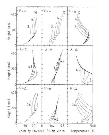
Fig.2.Some theoretical results of the open fire model.
The results are obtained for a 6-kW fire with excess air factor 1.8 and a volatile fraction of 0.8.
The parameters that have been varied in the calculations are mentioned in the specific graph.
The actual value prevailing in a fire has to be determined by experiment. As is to be expected, increase in excess air reduces maximum temperatures, increases flame heights, and reduces maximum velocities.
Two other parameters are of some relevance in determining the flame
behaviour. They are the mass fraction of volatiles leaving the fuelbed and
the fuelbed temperature. Figure 5.2 shows the influence of these parameters
on the fire behavior. According to Table 4.2 the volatile matter in wood
varies between 70 and 80%. Reducing the value to artificially low values
could be used as a simple means of modeling incomplete combustion of
volatiles. Incomplete combustion is a serious problem with solid fuel
burning. Emmons (1980) points out that flaming combustion burns only limited
fractions of the volatiles. For example, polystyrene foamed plastic burns
only 50% of the mass pyrolyzed; the remainder appears as a dense cloud of
soot, unburned and partially burned volatiles. The experiments on open wood
fires do not suggest this level of unburned volatiles. In connection with
this another factor needs to be kept in mind. In the present model, the
volatiles ratio in wood enters the calculation only through the
specification of the Froude number. A better method of modeling the effects
of incomplete combustion was not considered by Bussmann and Krishna Prasad.
The results in Fig. 2 show that reducing the volatiles does not produce
any unexpected result. The figure also includes the value of ![]() to
account for noncharring solids as well.
to
account for noncharring solids as well.
Finally, the fuelbed temperature has very little effect on the properties of the flaming combustion zone. This is as it should be since the Froude number reaches unity at the neck of the fire. The influences that occur in a region where the Froude number is less than unity will not propagate into regions where the Froude number is unity or greater. This raises the question about the role of the interface conditions on the flaming combustion zone. Two vital factors that are expected to strongly influence the interface conditions, namely, chemistry of the process and radiation, have been ignored in the present model. Thus the conclusions that could be derived here can at best be tentative.
Since the model is quite crude it requires experimental validation. The
results shown by Steward were all for much larger fires. The power levels of
the fire in those experiments were upward of 25 kW. Most of the wood fires
used for cooking applications at the domestic level would be in the range of
5 kW with the assumption that these fires can operate at efficiencies of
about 35%. The flame heights were measured for small wood fires by Bussmann
(1981) and Herwijn (1984). These are shown plotted in Fig.3 The results
were obtained with fires made on plain brick supports and a grate. In
general, power levels of the fire in these experiments were varied by
varying the base diameter of the fire. The flame heights were measured after
the fire appeared steady to an observer.
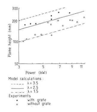
Fig.3. Flame heights: theory and experiment
5 Each point in the figure is the average of heights measured from 25 photographs taken at intervals of about three-fourths of a minute. The lines shown are obtained from the theory for different excess-air factors. Several interesting results emerge from the plots. First, the experiments without a grate agree with the theoretical result when the excess-air factor is about 2. The result of Steward(1970), as pointed out earlier, required a fourfold correction factor for agreement with experiment. This is attributed partially to the lower value of the entrainment coefficient chosen and partially to the manner in which the combustion process was incorporated into the model by Steward. Of course, there is the possibility that smaller fires might behave differently from bigger fires. Second, the grate fires exhibit larger flame heights than those without grates. They also agree reasonably with the theory for an excess-air factor of about 3. This is somewhat of an unexpected result. In general, a grate provides a better access to air in a fuelbed and in particular the burning of char is much better on a grate. Moreover, as the experimental results to be presented later suggest, a given area of grate is capable of providing a higher power level of fire than a corresponding fire without a grate. This result intuitively suggests that combustion intensity is higher with a grate and thus one could expect a lower combustion volume. However, the result suggests that the volume of flame without the grate is large. In Fig.4 we reproduce flame photographs obtained for the two cases for the same power level of the fire. The grate fire is tall and lean while the nongrate fire is short and stocky. In these experiments fire volumes were not measured. Visual inspection does not clearly indicate that the volume of the fire is larger with a grate.
There are several possible explanations for the fire behaviour described above. The first possibility is that for a grate fire the volatiles arrive at the flaming combustion zone in a greater premixed state and considerable combustion occurs in the core of the plume. This might affect the density gradient at the edge of the fire, thus adversely affecting the air entrainment. However, such an explanation is inconsistent with the theory of combustion in a fuelbed (see Section 4.3, Fig.4.7), which suggests that very little oxygen comes out of the fuelbed. But it must be pointed out that the results in Fig.4.7 are for forced draught combustion and the present work is for naturally ventilated fires.
The second possibility is that the fire over a grate is laminar while the nongrate fire is turbulent. The former will have a lower entrainment rate, thus leading to larger heights for completion of combustion. According to Corlett (1974) pool fires with diameters of the order of 10 cm or less are laminar while for base diameters of 100 cm or more they are turbulent. The pictures shown in Fig.4 are of fires with base diameters of 20 cm. Thus they may be in the transition regime and this leads to some questions about the applicability of our model to such fires. In view of our aim to keep things simple, we will ignore such questions. Unfortunately, this line of argument is unable to answer the question why a grate fire remains laminar while a nongrate fire of the same power level is either in the transition or the turbulent regime.
The third possible explanation is the conditions over a grate fire are correct for producing a fire whirl. The descriptions of such fire whirls caused by air raids over Hamburg during World War II are vivid (Lee and Hellman, 1974). Emmons (1965) describes an experimental arrangement for simulating fire whirls and Lee (1966) provides a theoretical description for the problem. The fire whirl is caused in a fire plume from an intense heat source by concentrating the ambient vorticity into a rapidly swirling vortex. Figure 5 shows two photographs taken with an apparatus with and without tangential air inlets to the flaming combustion zone. the grate fire bears a strong resemblance to the fire whirl photograph. More investigation is necessary to explain this phenomenon. This rather long discussion poses a series of intriguing problems about the difference between grate and nongrate fires. They require much more work, primarily of an experimental nature, to get a better understanding.
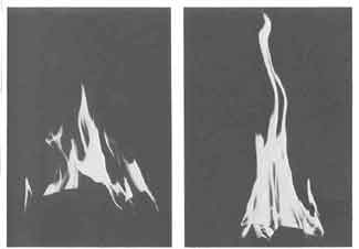
Fig.4. Flames from a wood fire with and without grate
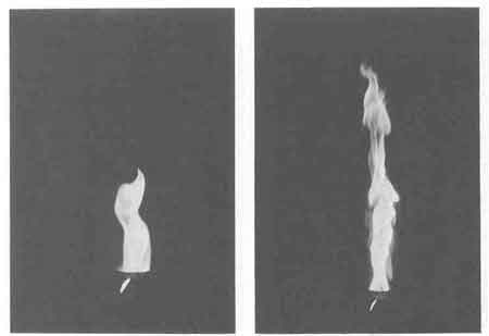
Fig.5.Flames from a kerosene fire with and without swirl-introducing equipment
We now return to Fig.3. A third result is that the flame height varies
with the power level of the fire according to the relation.
| (16) |
The power law in Eq.(5.13) is the same as the one found by Steward. C1 is a function of many parameters but for our purposes it is a strong function of the excess-air factor. For most fires the power density does not vary too much with the base area (Corlett 1974). Thus we can state that
| (17) |
Combining Eqs. (5.13) and (5.14), we obtain
| (18) |
For nongrate fires a reasonable value for power density appears to be about
20
![]() . In Eq.(5.15)
. In Eq.(5.15) ![]() is in centimeters.
is in centimeters.
Theories of this type provide useful guidelines for designing combustion chambers. From the experimental results it appears that for a naturally aspirated fire (without a grate) operating with an excess-air factor of 2 the combustion chamber height needs to be roughly equal to the base diameter of the fire for reasonably complete combustion. We shall have more to say on this dimension from the point of view of heat transfer in the next section.
Since the temperature profiles as a function of height are known from the theory, heat transfer estimates to the pan could be derived. The main reservation is that the theory as described here has many loopholes and is far too naive and needs to be used in close conjunction with experiment.
There has been very little work done on the measurement of temperatures in wood fires. However, the work of Cox and Chitty (1980) on simulated fire plumes produced by burning natural gas as diffusion flames on a porous refractory burner provides some useful insights into the validity of the theory. The axial velocity at the flame height level in their experiments correlated according to
| (19) |
[5~
The one-fifth power law is consistent with the height-power output relation
of Eq.(5.13). The constant ![]() was found from the experiments to be 1.867.
As pointed out earlier,
was found from the experiments to be 1.867.
As pointed out earlier, ![]() depends on the heating value of the fuel,
stoichiometric air/fuel ratio, and excess-air factor. Using an excess-air
factor of 2, as determined in the wood fire experiments (Cox and Chitty did
not report this quantity), calculations performed for natural gas with the
present model lead to a value of K equal to 1.633. The maximum temperature
according to these calculations was 1730 K while the measurements indicated
a value 1250 K.
depends on the heating value of the fuel,
stoichiometric air/fuel ratio, and excess-air factor. Using an excess-air
factor of 2, as determined in the wood fire experiments (Cox and Chitty did
not report this quantity), calculations performed for natural gas with the
present model lead to a value of K equal to 1.633. The maximum temperature
according to these calculations was 1730 K while the measurements indicated
a value 1250 K.
There are many reasons for the discrepancy between theory and experiment. The theory uses top-hat profiles and thus the difference between theory and prediction of velocity seems modest. However, there is a departure between theory and experiment for temperature, for which the difference is quite large. Cox and Chitty did not correct for radiation error in the measuring sensor. This error they estimated to be as high as 20% at the temperature level they were measuring. This brings the real flame temperature up to 1500 K. The present model does not account for radiation losses from the fire and some calculations presented in the next section show that these can account for about 8% of the energy content of the fuel for the class of fire we are considering. This, translated into temperatures, will be that predicted temperatures are about 100 K too high. The problem with the model is that it underpredicts velocity, but overpredicts the temperature. This may be due to the flat profiles used in the theory and the differences that might exist in diffusion of heat and momentum in turbulent flames. This requires further investigation. Thus the theory, while being very crude, with modest modifications, can be made to provide estimates of flame heights and temperatures which differ from reality by 10 to 15%. Such accuracies are probably quite adequate for the purposes of stove design.
The major weakness of the theory as it stands now is that it completely ignores the interaction between the fuelbed and fire plume. This might be important for developing suitable control of the power level of a stove.